2  Scattering theory

\[ \definecolor{C0}{RGB}{31, 119, 180} \definecolor{C1}{RGB}{255, 127, 14} \definecolor{MyBlue}{RGB}{0, 68, 136} \definecolor{MyYellow}{RGB}{221, 170, 51} \definecolor{MyRed}{RGB}{187, 85, 102} \]

The ultimate goal in particle physics is to understand how particles interact. Generally speaking, particle properties can only be studied by measuring cross sections in particle accelerator experiments, such as colliders or fixed-target experiments. We therefore need to relate the cross sections that are measured experimentally to a theory that describes the underlying particle reactions. In this chapter, we will see how scattering theory is the bridge that connects theory and experiment by giving us a means to formulate observable transition amplitudes.

2.1 The scattering matrix

Any particle reaction in an experiment can be reduced to a scattering process consisting of three stages [1]:

1. approach of the incoming particles (initial state),
2. a process of interaction, during which the incoming particles may scatter, temporarily form intermediate states, or transform into new sets of outgoing particles,
3. and the scattered or formed particles moving away (final state).

When the interaction stage (2.) occurs within a relatively short time, both the initial and final states can be treated as collections of free, non-interacting particles that are unaffected by the interaction potential. This is a reasonable assumption, because the interaction region is almost point-like in comparison to the detector size [1]. The non-interacting incoming and outgoing states may therefore be approximated as asymptotic states. The challenge then is to relate the incoming asymptotes to the outgoing ones by describing the interaction process. Importantly, whether describing a classical or a non-relativistic interaction potential, the scattering process is fully determined once the incoming and outgoing asymptotic states are specified. This requirement is known as the asymptotic condition.

In the classical picture, the scattering process can be visualised as in Figure 2.1. Far from the interaction region, the trajectory of the particle approaches a well-defined asymptote, which can be characterised by its incoming or outgoing momentum. Within the interaction region, the path of the particle is fully determined by the interaction potential. However, for most practical purposes, it is unnecessary to determine the trajectory to learn about the potential. Instead, one can define a continuous mapping that relates each incoming momentum to a corresponding outgoing momentum. Importantly, this mapping is expressed in terms of measurable momenta, offering insight into the underlying potential and, by extension, the Lagrangian that governs the system.

Figure 2.1: Sketch of the asymptotic condition in a classical scattering process. The connected continuum of incoming and outgoing momenta can be used to understand the interaction potential. Inspired by [1, Fig. 2.1].

In the quantum-mechanical case, the incoming and outgoing states are described by wave functions. Figure 2.2 is an artistic representation of that: an incoming plane wave travels through an interaction region where an approximately localised potential scatters it into a superposition of outgoing waves. In quantum mechanics, the interaction process is described in terms of an operator rather than a classical orbit. Wheeler first introduced the concept of a “collision matrix” [2], which Heisenberg formalised in the form of an \(\mathbf{S}\)‑matrix operator [3] (not to be confused with the spin operator). By abandoning the notion that the scattering process is to be described as a positional wave function, the scattering process is translated to a model of exact momentum states that can be related through operators in the Heisenberg picture. This better matches the observables that we measure in experiment [4; 5], where the experimentalist essentially prepares initial state wave packets in momentum space and measures the outgoing state as a distribution of four-momenta [6].

Figure 2.2: Scattering process of quantum mechanical wave functions. Incoming state \(\psi_\text{in}\) and outgoing state \(\psi_\text{out}\) are comparable to the asymptotes in Figure 2.1, but are defined as a superposition of quantum states in a specific basis of observables.

The idea of a scattering operator is quite general and can be applied to any scattering process, including particle decays, even if multiple decay channels are involved [7]. Consider such an arbitrary incoming state \(\ket{\psi_\text{in}}\). This can be any configuration of particles, such as \(e^-e^+\) about to collide. We want to find a description for the resulting outgoing state \(\ket{\psi_\text{out}}\) that can be a collection of decay products. Here, we introduce an \(\mathbf{S}\)‑matrix that maps the incoming state to the outgoing state by

\[ \Ket{\psi_\text{out}} \;=\; \mathbf{S}\Ket{\psi_\text{in}} \,. \tag{2.1}\]

This expression encodes the entirety of the interaction. Although the microscopic details of the dynamics may be complex or even unknown, the \(\mathbf{S}\)‑matrix summarises their net effect on the asymptotic particle states, which are accessible by experiments.

The \(\mathbf{S}\)‑matrix is an extremely general operator and has to be further specified depending on the particle reaction that is being studied. For instance, the dimension of the \(\mathbf{S}\)‑matrix represents the number of possible states of the initial and final state, which makes the \(\mathbf{S}\)‑matrix suitable for coupled channel studies. The \(\mathbf{S}\)‑matrix and the incoming and outgoing states also have to be further parametrised in terms of variables and quantum numbers that are of relevance to the experiment, such as collision energy, four-momenta, spin, parity, et cetera.

In practice, we separate the trivial part of the scattering process, where the incoming state passes through unaffected by the interaction potential, from the non-trivial part that contains the effects of the interaction. This leads to the decomposition

\[ \mathbf{S} \;=\; \mathbf{1} + i \mathbf{T}, \tag{2.2}\]

where \(\mathbf{1}\) is the identity operator (corresponding to no scattering) and \(\mathbf{T}\) is the transition operator. In some literature, the \(\mathbf{T}\)‑matrix is multiplied by a factor two, or a minus sign is used.

To relate these expressions back to experimental observables, we express the incoming and outgoing states in terms of observable basis states \(\ket{p_1,\dots,p_m;\alpha}\) and \(\ket{p_1',\dots,p_n';\beta}\), where \(p_i^{(\prime)}\) are the observable four-momenta of the particles, and \(\alpha, \beta\) label the set of discrete quantum numbers (such as spin, isospin, parity, and rest masses) that characterise the initial- and final-state channels. This leads to the transition matrix elements \(\mathcal{M}_{\!\beta\alpha}\) describing the process \(\alpha \to \beta\),

\[ \begin{aligned} & \Braket{p_1',\ldots,p_n';\beta|i\mathbf{T}|p_1,\ldots,p_m;\alpha} \\ & \quad =\; i (2\pi)^4 \, \delta^{(4)}\!\left(p_\beta - p_\alpha\right) \, \mathcal{M}_{\!\beta\alpha}\left(p_1, \dots; p_1', \dots\right) \,, \end{aligned} \tag{2.3}\]

where the \(\delta^{(4)}\)‑function ensures conservation of incoming and outgoing four-momenta, \(p_\alpha=p_\beta\), with \(p_\alpha=\sum_{i=1}^m p_i\) and \(p_\beta=\sum_{j=1}^n p_j'\). The quantity \(\mathcal{M}_{\!\beta\alpha}\) is called a “matrix element” because it represents a component of the transition operator \(\mathbf{T}\): it is the (discrete) projection into the transition \(\alpha \to \beta\) as a (continuous) function of their asymptotic incoming and outgoing four-momenta \(p_i^{(\prime)}\).

While the full \(\mathbf{S}\)‑matrix is a unitary operator acting on the entire Hilbert space of asymptotic momentum states [6], \(\mathcal{M}_{\!\beta\alpha}\) captures the physical content of a particular transition and is the quantity that enters into the calculation of cross sections, decay rates, and other observable quantities. It is a complex-valued amplitude function that encodes the likelihood of the process, with its modulus squared appearing in measurable rates. For instance, for a scattering process with \(n\) final-state particles, the differential cross section is given by

\[ \mathrm{d}\sigma_{\beta\alpha} \;=\; \frac{1}{F_\alpha} \left|\mathcal{M}_{\!\beta\alpha}\right|^2 \, \mathrm{d}\Phi_n \,, \tag{2.4}\]

where \(F_\alpha\) is a flux factor determined by the initial state \(\alpha\) and \(\mathrm{d}\Phi_n\) is the Lorentz-invariant phase space volume element [8, §49]

\[ \mathrm{d}\Phi_n \;=\; (2\pi)^4 \, \delta^{(4)}\!\left(p_\alpha-p_\beta\right) \prod_{i=1}^n \frac{\mathrm{d}^3 p_i'}{(2\pi)^3\,2E_i'} \tag{2.5}\]

for the \(n\)‑body final state. In decay processes, the cross section is often denoted with \(\mathrm{d}\Gamma\) rather than \(\mathrm{d}\sigma\) and is referred to as the partial or differential decay rate. The differential cross section quantifies the probability density for the transition from the initial state \(\alpha\) to the final state \(\beta\), as a function of the kinematic degrees of freedom in the final state and of the configuration of the initial state.

The matrix elements \(\mathcal{M}_{\!\beta\alpha}\) denote the momentum projection of the transition operator \(\mathbf{T}\) and are, as such, continuous functions of the incoming and outgoing momenta. In practice, we prefer to parametrise transition matrix elements as a function of other kinematic variables that are more relevant to the reaction process. The implicit convention in literature is to call such functions transition amplitudes and we follow the conventional notation to denote these functions with \(A\) or \(a\). Amplitudes are like the response functions that tell how a system responds to external perturbations [9, p. 274], and the fact that they are directly related to observable cross sections makes them a powerful experimental tool for extracting information about the underlying dynamics of particle interactions.

2.2 \(\mathbf{S}\)‑matrix constraints

In theory, it is impossible to derive proper parametrisations of scattering amplitudes directly from the full QCD Lagrangian. The non-perturbative nature of the strong coupling at low energies makes exact solutions intractable. We can, however, derive a few basic constraints for the \(\mathbf{S}\)‑matrix from fundamental principles of quantum mechanics and special relativity. These constraints are universal and model-independent: they must be satisfied by any theory of scattering, including QCD.

From this perspective, the \(\mathbf{S}\)‑matrix provides an alternative but complementary framework to QCD – even though it historically preceded the concept of QCD itself [4, §7.1]. Rather than describing the microscopic dynamics of quarks and gluons, it focuses on observable relations between asymptotic states. The \(\mathbf{S}\)‑matrix formalism enables amplitude models that enforce general physical principles while remaining agnostic about underlying dynamics, and provides a bridge between QCD predictions and experimental observables in the hadronic regime [10]. The most commonly invoked constraints are Lorentz invariance, unitarity of the transition amplitudes, and crossing symmetry.

Lorentz invariance

Given that we describe scattering entirely in terms of the momenta of incoming and outgoing particles, we must ensure that this description remains consistent under any change of inertial frame, so that we can relate it to the laboratory frame in which we perform our measurements. This requirement of relativistic invariance reflects the symmetry of spacetime as described by special relativity. Any theoretical description of scattering must respect the fact that the outcome of a physical process should not depend on the inertial frame in which it is described.

In relativistic quantum mechanics, this requirement is implemented through the Poincaré group, which comprises both spacetime translations and Lorentz transformations (rotations and boosts). The \(\mathbf{S}\)‑matrix must commute with the generators of this symmetry group to ensure that they transform appropriately under changes of frame. In particular, Lorentz invariance implies that the \(\mathbf{S}\)‑matrix must be invariant under Lorentz transformations. If we define \(\mathbf{U}\) as the unitary transformation that maps a Lorentz transformation \(\boldsymbol{\varLambda}\) to the corresponding operator acting on the Hilbert space of quantum states, Lorentz invariance implies that

\[ \mathbf{U}[\boldsymbol{\varLambda}] \; \mathbf{S} \; \mathbf{U}^\dagger[\boldsymbol{\varLambda}] \;=\; \mathbf{S} \,. \]

This constraint has important practical implications. First, it means that scattering amplitudes can only be a function of Lorentz-invariant combinations of the asymptotic four-momenta. Second, Lorentz invariance constrains how spin degrees of freedom must be treated. In a non-relativistic regime, spins can be added using standard angular momentum algebra, but the transformation of spin states under boosts becomes non-trivial (Chapter 3).

Unitarity

The most natural constraint is that the transition preserves probability, that is, ‘what comes in, comes out’. In the notation of Equation (2.1), this means

\[ \begin{aligned} \Braket{\psi_\text{in}|\psi_\text{in}} \;&=\; \Braket{\psi_\text{out}|\psi_\text{out}} \\ \;&=\; \Braket{\psi_\text{in}|\mathbf{S}^\dagger\mathbf{S}|\psi_\text{in}} \,, \end{aligned} \]

which gives us the unitarity condition that ensures that the total probability for any process remains normalised,

\[ \mathbf{S}^\dagger \mathbf{S} \;=\; \mathbf{S}\mathbf{S}^\dagger \;=\; \mathbf{1} \,, \]

with \(\mathbf{1}\) the identity matrix. Inserting Equation (2.2) gives us the unitarity condition for the \(\mathbf{T}\)‑matrix,

\[ \mathbf{T} - \mathbf{T}^\dagger \;=\; i \mathbf{T}^\dagger \mathbf{T} \,. \tag{2.6}\]

This equation shows that the imaginary part of the transition amplitude is constrained by its own modulus. Physically, it implies that the scattering process may involve not just direct deflection, but also the temporary formation of intermediate states such as resonances (elastic scattering), or transitions into entirely different final states (inelastic scattering) that are not accounted for in the model. In elastic scattering, the imaginary part of the amplitude reflects the finite lifetime of the resonant state, while in inelastic scattering, it indicates a genuine loss of flux from the initial channel into other open channels. Both effects are captured by the complex structure of the \(\mathbf{T}\)‑matrix, and its imaginary part plays a central role in encoding how probability is redistributed across scattering channels. In Section 2.4, we will see how this leads to observable phase shifts in the scattering amplitude.

Analyticity

In any physical process, causes must precede their effects. In scattering theory, causality requires that the wave function of a particle cannot “respond” before the interaction has taken place. This causal requirement leads to a mathematical condition: the transition matrix elements \(\mathcal{M}_{\!\beta\alpha}\) must be analytic in energy and momentum, meaning that the energy-momentum domain can be continued into the complex plane and that it varies in a way that is smooth, except at well-defined singularities associated with physical thresholds or states.

The connection between causality and analyticity becomes more transparent when we recognise that the \(\mathbf{S}\)‑matrix relates asymptotic momentum states in a way that is analogous to how a Fourier transform relates position and momentum space. Just as a time-localised function has a smooth (analytic) Fourier transform in frequency space, a localised interaction in spacetime leads to an analytic amplitude function in energy space [11; 9, p. 390]. This analyticity implies that the amplitude as a function of energy can be extended to a complex plane, where singularities such as poles appear in specific regions. These poles correspond to physical phenomena like bound states or resonances. While bound states appear as poles on the real axis, unstable states (resonances) correspond to poles with a negative imaginary part. Causality ensures this sign: it guarantees that the amplitude decays as time increases. A pole in the upper half-plane (positive imaginary part) would imply that the amplitude grows with time, violating the principle that effects cannot precede causes.

Analyticity gives the scattering amplitude an internal structure that causes it to “feed back” into itself – its absorptive component is determined by how likely it is to scatter into other channels, which is itself encoded in the amplitude. This enables powerful tools such as dispersion relations, which relate the value of an amplitude at one energy to its values elsewhere [12]. Once we know the amplitude in one location, we can analytically continue it through the complex plane into other regions of interest. Since the interaction potential is itself governed by the underlying fundamental forces, these relations allow us to extract information about the dynamics from measured cross sections, and compare them to those predicted by the formulated amplitude model [13].

Crossing symmetry

Scattering processes can be visualised with Feynman diagrams, which represent terms in the perturbative expansion of the \(\mathbf{S}\)‑matrix. A striking feature is that a single Feynman diagram can often describe multiple processes. For instance, the diagram representing a 2-to-2 scattering process \(A + B \to C + D\) can, under certain momentum substitutions, also describe \(A + \bar{C} \to \bar{B} + D\). This observation reflects a property of QFT known as crossing symmetry. Once this additional constraint is combined with the unitarity and analyticity conditions, the transition amplitudes of seemingly unrelated reactions become connected representations of a single analytic object that is a manifestation of the underlying field theory [9, p. 274; 14; 15].

Crossing symmetry was first described by Mandelstam [16], in a paper that also introduced the Mandelstam variables, or invariants, which provide a Lorentz-invariant description of two-body scattering kinematics. For a process \(A+B \to C+D\), they are defined as

\[ \begin{alignedat}{3} s \;&=\; (p_A + p_B)^2 \;&&=\; (p_C + p_D)^2 \\ t \;&=\; (p_A - p_C)^2 \;&&=\; (p_D - p_B)^2 \\ u \;&=\; (p_A - p_D)^2 \;&&=\; (p_C - p_B)^2 \,, \end{alignedat} \tag{2.7}\]

where \(p_A,p_B\) are the four-momenta of the incoming particles and \(p_C,p_D\) those of the outgoing particles. Here, \(s\) combines the incoming momenta as a sum, giving the squared center-of-mass energy, while \(t\) and \(u\) involve momentum differences and measure the momentum transfers between initial and final states. The difference in structure indicates two distinct reaction types: \(s\) characterises a “direct” reaction, in which the two incoming momenta combine, whereas \(t\) and \(u\) characterise “exchange” reactions that pair an incoming with an outgoing leg and describe momentum exchange (see Figure 2.3).

Figure 2.3: The two reaction types that can be distinguished in a 2-to-2 scattering process.

Each of these variables is often associated with a distinct channel topology or Feynman diagram (see Figure 2.4), which complements their broader role as analytic variables of the full 2-to-2 amplitude. The \(s\)‑channel corresponds to the configuration in which the two incoming particles are combined, with \(s\) equal to their squared invariant mass. The \(t\)‑channel corresponds to the configuration in which an incoming particle is paired with one of the outgoing particles, characterised by the squared momentum transfer \(t\). The \(u\)‑channel corresponds to the alternative pairing, where each incoming particle is combined with the other outgoing particle, giving the squared momentum transfer \(u\). By crossing symmetry, an incoming particle can be reinterpreted as an outgoing antiparticle, which reverses the sign of its momentum.

Figure 2.4: Channel topologies that are often associated with the three Mandelstam variables \(s\), \(t\), and \(u\) in a 2-to-2 scattering process in terms of the four-momenta of the incoming particles \(A\) and \(B\) and outgoing particles \(C\) and \(D\). Momenta on the same side of the diagram contribute with a plus sign, while those on opposite sides contribute with a minus sign.

This perspective also clarifies how Mandelstam invariants appear in three-body decays. If a three-body final state is viewed as a sequence of two-body subprocesses, the same diagrammatic topologies reappear when deforming the scattering diagrams of Figure 2.4 into the decay diagrams of Figure 2.5. In this case, particle \(B\) is no longer incoming but part of the final state, so its momentum enters with the opposite sign. The resulting invariants are just the squared masses of two-body subsystems, which play the same role in Dalitz-plot analyses of decays as the Mandelstam variables do in scattering.

Figure 2.5: Mandelstam variables defined in the two-body subsystems of a three-body decay, obtained from the scattering topologies of Figure 2.4 by reinterpreting incoming particle \(B\) as part of the final state. In this decay picture, all momenta that enter a given invariant lie causally on the same side of the process and therefore appear with a plus sign.

Because of four-momentum conservation, the Mandelstam variables are not independent but satisfy

\[ \begin{aligned} s + t + u \;&=\; p_A^2 + p_B^2 + p_C^2 + p_D^2 \\ \;&=\; m_A^2 + m_B^2 + m_C^2 + m_D^2 \,, \end{aligned} \tag{2.8}\]

A 2-to-2 scattering process can therefore be described in terms of only two independent invariants. This already hints that the processes sketched in Figure 2.4 and Figure 2.5 are not isolated but intrinsically connected.

These connections are visualised in Figure 2.6, which plots the Mandelstam variables over a real-valued, two-dimensional Mandelstam plane. The plot uses a barycentric coordinate system, with \(x=\frac{s-t}{(s+t+u)\sqrt{2}}\) and \(y=\frac{s+t-2u}{(s+t+u)\sqrt{6}}\), to emphasise that the choice of \(s\), \(t\), and \(u\) is arbitrary and that the three variables are symmetrically related to each other through Equation (2.8). The yellow regions mark the values kinematically allowed for given particle masses \(m_A, m_B, m_C, m_D\), that is, the regions where experimental measurements can be made. They are determined by the condition that the Kibble function [17]

\[ \phi(s,t,u) \;=\; \lambda\!\left( \lambda(s, m_B^2, m_A^2),\, \lambda(t, m_C^2, m_A^2),\, \lambda(u, m_D^2, m_A^2) \right) \tag{2.9}\]

is negative [9, pp. 175–177]. Here, \(\lambda\) denotes the Källén function [18, pp. 11–12], a symmetric polynomial in three variables, defined as

\[ \lambda(x,y,z) \;=\; x^2 + y^2 + z^2 - 2xy - 2yz - 2zx \,. \tag{2.10}\]

Now, although these kinematically allowed regions are disjoint, and their Feynman diagrams correspond to distinct physical reactions, crossing symmetry tells us that they are analytically connected. Each scattering or decay channel corresponds to a different real slice of the same complex analytic function \(A(s,t,u)\). What appear experimentally as separate processes are therefore a mere set of boundary values of one underlying analytic structure (“Mandelstam Hypothesis” [16; 19; 20, §III; 9, p. 274]).

Figure 2.6: Barycentric visualisation of the kinematically allowed regions (shaded yellow) in the Mandelstam plane. The arrows indicate that the transition amplitudes for each reaction are connected through analytic continuation in the complexified plane. In this example, the regions are asymmetric, because each of the rest masses are all chosen differently.

Figure 2.6 also shows that, unlike in scattering, the three topologies of a three-body decay all occupy the same physical region. As we will see later, the amplitude can be expressed in terms of leading-order two-body subsystems, which are realised simultaneously in the Dalitz plot. This decomposition simplifies the analysis, but only approximates the full crossing-symmetric amplitude, since truncating the two-body partial-wave expansion (Section 2.3) inevitably violates exact crossing symmetry.

By modelling three-body decays as a sequence of two-body decays (Figure 2.5), the transition amplitude can be split into separate amplitudes that are parametrised as a function of a Mandelstam variable and a corresponding scattering angle \(\theta\) (Chapter 3), giving us

\[ A_{\text{total}}(s,t,u) \;=\; A^{(s)}(s,\theta_s) + A^{(t)}(t,\theta_t) + A^{(u)}(u,\theta_u) \,, \tag{2.11}\]

with \(A^{(s)}, A^{(t)}, A^{(u)}\) the amplitudes of the individual subsystems and \(\theta_s, \theta_t, \theta_u\) the corresponding scattering angles. Since \(\theta\) can itself be written in terms of another Mandelstam variable (Equation (2.26)), the angular part acquires a dynamical component that is analytically connected to the other channels.

A fully crossing-symmetric amplitude \(A(s,t,u)\) that is analytic in the three Mandelstam variables simultaneously is in principle the ideal objective, but constructing such an object is extremely challenging [21]. The Khuri–Treiman formalism [22] starts from Equation (2.11) and refines the partial amplitudes through dispersion-relation corrections constrained by analyticity and two-body scattering data. The method has no fundamental restriction to non-zero spin, but its extension to a spinful final state is technically demanding. Regge theory is also relevant to the broader programme of constructing crossing-symmetric amplitudes, as it analytically continues the discrete angular momenta in the partial-wave expansion to complex values [23].

2.3 Partial-wave expansion

In Section 1.1, we saw that many of the quantum numbers used to classify hadrons – such as spin, parity, and total angular momentum – stem from the symmetries of space and time. For example, spin and orbital angular momentum arise from rotational invariance, while parity is associated with spatial inversion symmetry. These symmetry-related quantum numbers remain relevant in scattering theory, where they constrain the allowed transitions between incoming and outgoing states.

This is the key idea: if the system is rotationally invariant, then the total angular momentum must be conserved. Each amplitude component with a specific total angular momentum therefore scatters independently. The case of two-particle scattering \(A+B \to C+D\) again makes this particularly clear. The sum of the momenta of the incoming particles defines a preferred direction, typically taken to be the \(z\) axis. Once we boost into the center-of-mass (CM) frame, and consider a fixed total energy \(s\) (Equation (2.7)), the geometry of the scattering process can be captured purely in terms of two angles, the scattering angle \(\theta\) (angle between \(p'_C\) and \(z\) axis, see Figure 2.7) and the azimuthal angle \(\phi\) (angle between the \(p'_A p'_B\) plane and \(p'_Cp'_D\) plane). Indeed, once \(s\) is fixed, only rotational degrees of freedom remain, so any structure in the amplitude at fixed energy must reflect how the interaction redistributes angular momentum across different scattering angles.

Figure 2.7: The sum of the incoming four-momenta can be used to define a \(z\) axis in the laboratory frame (left) and to boost into the CM frame (right). For a given total energy \(s\), the four-momenta in the CM frame define the scattering angle \(\theta\) (shown in the figure) and the azimuthal angle \(\phi\) (not shown).

Similar to how a sound wave can be decomposed into pure tones of different frequencies, the amplitude \(A(s, t)\) can be decomposed into independent (orthogonal) functions over the scattering angles. The result is called a partial-wave expansion [9, §4.4; 1, §6–c]. When the scattered particles have no intrinsic spin, these functions are given by the Legendre polynomials \(P_\ell(\cos\theta)\) that depend only on the scattering angle \(\theta\). The amplitude at fixed total energy \(s\) can then be written as a sum over the orbital angular momenta \(\ell\),

\[ A(s,\theta) \;=\; \sum_{\ell=0}^{\infty} (2\ell + 1) \, P_\ell(\cos\theta) \, a^{(\ell)}(s) \,. \tag{2.12}\]

Here, \(a^{(\ell)}(s)\) are the partial-wave amplitudes that encode the strength of the interaction in the orbital angular-momentum channel \(\ell\) purely as a function of energy \(s\). Overall, this is a Fourier–Legendre expansion, where \(P_\ell\) plays the role of orthogonal basis functions.

In order to generalise the partial-wave expansion to particles of arbitrary spin, we need to introduce a few additional quantum numbers. If the incoming and outgoing particles \(i=\{A,B,C,D\}\) have spin state \(\ket{J_i,\lambda_i}\), with \(\lambda_i\) the spin projection of particle \(i\) along some quantisation axis, the amplitude can be projected into independent amplitudes \(A_{\{\lambda\}}(s,\theta,\phi)\), with \(\lambda=\{\lambda_A,\lambda_B;\lambda_C,\lambda_D\}\). These amplitudes can be expressed in terms of total angular momenta \(J\) (coupled basis of total spin and orbital angular momentum), so that the expansion coefficients become a matrix of functions of both \(\theta\) and \(\phi\) [24, p. 413],

\[ \begin{aligned} A_{\{\lambda\}}(s,\theta,\phi) \;&=\; \sum_{J} (2J + 1) \, D^{J\,*}_{\mu \mu'}(\phi, \theta, 0) \, a^{(J)}_{\{\lambda\}}(s) \\ \;&=\; e^{i(\mu-\mu')\phi} \, \sum_{J} (2J + 1) \, d^J_{\mu \mu'}(\theta) \, a^{(J)}_{\{\lambda\}}(s) \,, \end{aligned} \tag{2.13}\]

with \(\mu=\lambda_A-\lambda_B\) and \(\mu'=\lambda_C-\lambda_D\). The Wigner \(D\)‑ and \(d\)‑functions are the matrix elements of rotation operators in the spin‑\(J\) representation that generalise the Legendre polynomials for the spinless case. We return to the relation between the Wigner functions, the helicity basis, and the canonical spin basis in Chapter 3. If the scattered particles have no intrinsic spin, the total angular momentum \(J\) equals the orbital angular momentum \(\ell\), and the familiar expansion of Equation (2.12) is recovered from Equation (2.13), because for any angles \(\alpha,\beta,\gamma\),

\[ D^\ell_{0,0}(\alpha,\beta,\gamma) \;=\; d^\ell_{0,0}(\beta) \;=\; P_\ell(\cos\beta) \,. \]

The key point is that we have factorised the transition amplitude \(A(s,t)\) into (1) angular components that we know how to parametrise as a function of angles and (2) dynamic partial-wave amplitudes \(a^{(J)}_{\left\{\lambda\right\}}(s)\) that are purely energy-dependent. By orthogonality, these dynamic partial-wave projections are given by the inverse of Equation (2.12) and Equation (2.13),

\[ \begin{aligned} a^{(\ell)}(s) \;&=\; \frac{1}{2} \int_{-1}^{1}\! \mathrm{d}(\cos\theta) \, P_\ell(\cos\theta)\,A(s,\theta) \\ a^{(J)}_{\{\lambda\}}(s) \;&=\; \frac{1}{4\pi}\! \int_{-1}^{1}\! \mathrm{d}(\cos\theta) \int_{0}^{2\pi}\! \mathrm{d}\phi \, D^J_{\mu\mu'}(\phi,\theta,0)\, A_{\{\lambda\}}(s,\theta,\phi) \,. \end{aligned} \tag{2.14}\]

For convenience, we often drop the quantum numbers \(\ell\), \(J\), and \(\{\lambda\}\), so that \(a(s)\) refers to a partial-wave amplitude. In Section 2.4, we will model this dynamic function \(a(s)\) in order to extract information about the interaction potential from experimental data. Right now, however, we can already further constrain this energy-dependent parametrisation purely on kinematic grounds.

As a first step, the factorisation into partial waves simplifies the unitarity condition on the transition matrix. When projected onto the angular momentum eigenbasis, Equation (2.6) becomes an energy-dependent condition that works separately for each \(J\). By applying Equation (2.3) to Equation (2.6), we get the unitarity condition for the matrix elements,

\[ \mathcal{M}_{\!\beta\alpha} - \mathcal{M}_{\!\alpha\beta}^* \;=\; i(2\pi)^4 \, \sum_{\gamma}\delta^{(4)}\!\left(p_\alpha - p_\beta\right) \, \mathcal{M}_{\!\gamma\beta}^* \, \mathcal{M}_{\!\gamma\alpha} \,, \tag{2.15}\]

where \(\gamma\) runs over all considered transition channels. This is known as the generalised optical theorem [25, p. 512; 6, p. 147]. Reformulating Equation (2.15) in terms of Lorentz-invariant variables \(s,t\) and applying the partial-wave projection from Equation (2.14), we get an energy-dependent unitarity condition for the partial-wave amplitudes,

\[ \operatorname{Im}a_{\beta\alpha}(s) \;=\; \sum_{\gamma} a_{\gamma\beta}^*(s) \, \rho_\gamma(s) \, a_{\gamma\alpha}(s) \,, \tag{2.16}\]

or, in matrix form,

\[ \operatorname{Im}\mathbfit{a}(s) \;=\; \mathbfit{a}^\dagger(s) \, \mathbfit{\rho}(s) \, \mathbfit{a}(s) \,. \tag{2.17}\]

In the single-channel case, this partial-wave unitarity condition becomes a more recognisable form of the optical theorem,

\[ \operatorname{Im} a(s) \;=\; \rho(s)\,\left|a(s)\right|^2 \,, \tag{2.18}\]

which relates the imaginary part of the partial-wave amplitude to its cross section. Here, we have introduced a Lorentz-invariant, normalised phase space factor \(\rho(s)\). In general, this factor is defined as the integral of the phase space element of Equation (2.5) over the angular degrees of freedom at fixed total centre-of-mass energy \(s\). In the special case of two-body scattering or decays, this integral has an analytic solution and can be expressed in terms of the breakup momentum \(q(s)\) [8, §50, p.8],

\[ \rho(s) \;=\; 4 (2\pi)^5 \int\mathrm{d}\Phi_2 \;=\; \frac{2q(s)}{\sqrt{s}} \;=\; \frac{\sqrt{\lambda(s, m_C^2, m_D^2)}}{s} \,. \tag{2.19}\]

The factor \((2\pi)^4\) is often absorbed into \(\Phi\), leaving a conventional factor \(8\pi\).The precise form of Equation (2.18) also depends on the normalisation of the scattering amplitude: with the convention of Equation (2.4), the inverse amplitude satisfies \(\operatorname{Im} a^{-1}(s) = \rho(s)\), while alternative normalisations shift factors such as \(16\pi\) into the definition of \(\rho(s)\).

The appearance of \(\lambda\) from Equation (2.10) reflects the same kinematic constraint \(\phi(s,t,u)<0\) of Equation (2.9) that defines the boundary of the physical region in Mandelstam space (see Figure 2.6). The phase space factor \(\rho(s)\) thus plays the role of an energy-dependent normalisation, arising directly from unitarity and the kinematics of the two-body system.

As a reminder, when working with multiple channels, a subscript in the phase space factor or breakup momentum indicates the channel for which it is defined. For a two-body final state \(\alpha\) with rest masses \(m_{1,\alpha}, m_{2,\alpha}\), this means

\[ \begin{aligned} \rho_\alpha(s) \;&=\; \frac{\sqrt{s-(m_{1,\alpha}-m_{2,\alpha})^2}\sqrt{s-(m_{1,\alpha}+m_{2,\alpha})^2}}{s} \\ q_\alpha(s) \;&=\; \frac{\sqrt{s-(m_{1,\alpha}-m_{2,\alpha})^2}\sqrt{s-(m_{1,\alpha}+m_{2,\alpha})^2}}{2\sqrt{s}} \,. \end{aligned} \tag{2.20}\]

This form with a product of square roots is often preferred over Equation (2.19), as it has a simpler analytic structure in the complex plane (one branch cut, see Section 2.4.4).

Unitarity also motivates a useful parametrisation of the partial-wave amplitudes in terms of a phase shift. We can rewrite Equation (2.18) to

\[ \left|1+i\rho(s)\,a(s)\right| \;=\; 1 \,, \]

which confines \(\rho(s)\,a(s)\) to a circle in the complex plane. Positions on that circle can be associated to angles, which naturally leads to parametrising the amplitude in terms of a phase shift \(\delta(s)\) via

\[ \begin{aligned} & a(s) \;=\; \frac{e^{2i\delta(s)} - 1}{2i \, \rho(s)} \\ & \Rightarrow \; e^{i\delta(s)} \sin\delta(s) \;=\; \rho(s) \, a(s) \,. \end{aligned} \tag{2.21}\]

Physically, \(\delta(s)\) represents the delay of the outgoing wave relative to free propagation. Its behaviour as a function of energy reveals features such as resonances and bound states – a rapid increase in \(\delta(s)\) indicates elastic effects during the scattering process.

As a first step in a partial-wave analysis (PWA), one often applies the partial-wave expansion without committing to any detailed dynamical model of \(a(s)\). In practice, the experimental data is divided into bins of the energy variable \(s\). Within each bin, one assumes that \(s\) is effectively constant and that the corresponding partial-wave amplitude \(a^{(\ell)}(s)\) can be approximated by a single complex parameter. The angular distribution observed in that bin is then fitted by adjusting these complex coefficients, one for each included partial wave. Each coefficient is thus treated as a free parameter of the fit, with no energy dependence imposed across bins.

The result is a collection of complex values \(\{a^{(\ell)}(s_i)\}\) at the bin centers \(\{s_i\}\). If these values vary smoothly from bin to bin, they can be interpolated to define a continuous amplitude function, from which phase shifts can be extracted. Such model-independent or energy-independent PWAs [26] already provide valuable insight into resonant behaviour, since characteristic phase motions across the energy range can already reveal the presence of resonant structures without assuming any specific parametrisation.

2.4 Resonance identification

When we visualise measured cross sections as a function of energy, we often observe sharp peaks or dips at specific energies. An example is shown in Figure 2.8, which displays the differential cross section for three backward-angle pion–nucleon scattering processes (\(\pi^+p \to \pi^+p\), and \(\pi^-p \to \pi^-p\), and \(\pi^-p \to \pi^0n\)). The curves represent fitted amplitude analyses that combine data from several pion–proton scattering experiments [26]. The observed structures reflect the underlying dynamics of the strong interaction. Scattering experiments are therefore like probing a bell, where the peaks correspond to the characteristic frequencies at which the bell resonates. The width of these peaks indicates how long the bell rings before returning to equilibrium, which in the scattering case is related to the lifetime of the excited state. In hadron physics, such structures are interpreted as resonances – unstable states that exist for a finite time before decaying into other particles.

Figure 2.8: Differential cross sections \(\mathrm{d}\sigma/\mathrm{d}\Omega\) for three different pion–nucleon scattering processes at the backward scattering angle (\(\theta=180^\circ\)). Shown are two fitted solutions based on amalgamated data from several pion–proton scattering experiments. Adapted from [26, Fig. 10].

Equation (2.4) allows us to relate the observable cross section distribution to the matrix elements \(\mathcal{M}_{\!\beta\alpha}\) and Equation (2.13) helps us to further split up the cross section into partial-wave amplitudes \(a^{(J)}(s)\) for each total angular momentum \(J\). The bumps will now only appear in certain total angular momentum channels, which we can identify by looking at the phase shifts \(\delta(s)\) of the partial-wave amplitudes. This suggests that the resonances are actual particles with an intrinsic spin that couples to that total angular momentum.

In certain processes, such as pion–nucleon scattering, one can go beyond spin and angular momentum and also extract the isospin of the resonances. The individual charge channels shown in Figure 2.8 are not themselves states of definite isospin, but fixed linear combinations of the \(I=\tfrac{1}{2}\) and \(I=\tfrac{3}{2}\) amplitudes. A partial-wave analysis of a single channel therefore cannot separate the isospin components. Only by fitting the elastic reactions \(\pi^+p\) and \(\pi^-p\) together with the charge-exchange channel \(\pi^-p\to\pi^0n\) can one extract information about the isospin amplitudes. This coupled-channel treatment makes it possible to disentangle the isospin structure of the partial waves and to assign resonances their total isospin.

For \(\pi N\) scattering the situation is relatively simple, since the initial state can only be in an \(I=\tfrac{1}{2}\) or \(I=\tfrac{3}{2}\) configuration. The relation between the observable charge channels and the isospin amplitudes is \[ \begin{aligned} \pi^+ p \to \pi^+ p \; &: \; A_{3/2} \\ \pi^- p \to \pi^- p \; &: \; \tfrac{1}{3} A_{3/2} + \tfrac{2}{3} A_{1/2} \\ \pi^- p \to \pi^0 n \; &: \; \tfrac{\sqrt{2}}{3}\left(A_{3/2} - A_{1/2}\right) \;, \end{aligned} \]

where \(A_{1/2}\) and \(A_{3/2}\) denote the partial-wave amplitudes with definite isospin. While the details of this isospin decomposition are beyond the scope of this work, it helps to understand what certain partial-wave labels mean and how these waves are extracted. For example, the \(P_{33}\)‑wave (Figure 2.9) denotes for a partial wave with orbital angular momentum \(\ell=1\), isospin \(I=\tfrac{3}{2}\), and total angular momentum \(J=\tfrac{3}{2}\), and how they are extracted from total differential cross sections. Similarly, the \(D_{15}\)‑wave corresponds to \(\ell=2\), \(I=\tfrac{1}{2}\), and \(J=\tfrac{5}{2}\). The scheme follows spectroscopic letter notation \(S,P,D,F,\dots\) for orbital angular momentum \(\ell=0,1,2,3,\dots\).

Figure 2.9 shows the imaginary and real parts of the \(P_{33}\)‑wave obtained from the pion–nucleon cross sections of Figure 2.8 [27]. The prominent peak around \(1.23\ \text{GeV}\) and the zero-crossing of the imaginary part reveals the \(\varDelta(1232)\) resonance with quantum numbers \(I\left(J^P\right)=\tfrac{3}{2}\left(\tfrac{3}{2}^+\right)\). This is a striking example of how resonances emerge from the partial-wave amplitudes: once hidden in the energy spectrum, they stand out clearly in the complex amplitude. The remainder of this section introduces the techniques that make such extractions possible.

Figure 2.9: Real and imaginary part of the \(P_{33}\)‑wave amplitude that was extracted from the pion–nucleon scattering cross section in Figure 2.8. The position of the peak of one of the three bumps is highlighted in red. Adapted from [27, Fig. 3].

Breit–Wigner parametrisation

To model the shape of a resonance, we need a function that captures both the peak structure and a width that is associated with the lifetime of the resonance. A simple but remarkably effective parametrisation is the Breit–Wigner function [28], which describes the relativistic scattering amplitude near a resonance as a function of energy \(s\),

\[ a(s) \; \cong \; \frac{1}{M_R^2 - i M_R \Gamma_R - s} \,, \tag{2.22}\]

where \(M_R\) is the mass of the resonance and \(\Gamma_R\) its total decay width. The numerator often includes a scaling factor or is normalised to the peak by setting it equal to \(M_R\Gamma_R\), but these factors are left out here (indicated by \(\cong\)). This functional form mirrors the response of a driven, damped harmonic oscillator – a system that resonates when driven near its natural frequency but loses energy due to damping. Similarly, the Breit–Wigner function reflects how the system “rings” in response to a scattering event and then decays.

Figure 2.10 visualises the Breit–Wigner function through its modulus squared, real and imaginary parts, and the associated phase. The resonance appears most clearly in the left panel, where the modulus \(|a_J|^2\) forms its characteristic peak at \(s = M_R^2\) with a finite width controlled by the imaginary term \(iM_R\Gamma_R\) in the denominator. The Argand diagram in the middle plots \(\operatorname{Im}a_J\) against \(\operatorname{Re}a_J\) to show how an isolated Breit–Wigner traces out a circle, thereby preserving unitarity with inelasticity \(\eta=1\). The same diagram also highlights the connection between the phase shift \(\delta(s)\) of Equation (2.21) and the modulus of the amplitude. The right panel shows that the corresponding phase shift \(\delta(s)\) undergoes a rapid increase by approximately \(\pi\) across the resonance region, which indicates a relative time delay of the outgoing wave.

import os

import matplotlib.pyplot as plt
import numpy as np
from matplotlib import patches

plt.ioff()
plt.rc("font", family="serif", serif="Helvetica", size=13)
plt.rc("mathtext", fontset="dejavusans")
plt.rc("text", usetex=True)

def breit_wigner(s, m0, w0):
    return 1 / (m0**2 - 1j * m0 * w0 - s)


def bw_delta(s, m0, w0):
    bw = breit_wigner(s, m0, w0)
    norm = np.abs(breit_wigner(m0**2, m0, w0))
    return np.angle(1 + 2j * bw / norm) / 2


m0 = 1.0
Γ0 = 0.25
R = 0.55
s = np.linspace(0, 2, num=1000)
bw = breit_wigner(s, m0, Γ0)

fig, axes = plt.subplots(figsize=(7, 2.1), ncols=3)
fig.subplots_adjust(bottom=0, left=0, right=1, top=1, wspace=0.12)
ax1, ax2, ax3 = axes
fig.patch.set_facecolor("none")
for ax in axes:
    ax.patch.set_facecolor("none")
    ax.spines["left"].set_position("zero")
    ax.spines["bottom"].set_position("zero")
    ax.spines["top"].set_visible(False)
    ax.spines["right"].set_visible(False)

ax1.axvline(m0**2, color="#e6332a", ls="dashed", lw=1.5, zorder=-10)
ax1.text(
    x=m0**2 - 0.05,
    y=-0.5,
    s=R"$M_R^2$",
    color="#e6332a",
    ha="right",
    va="top"
)
ax1.plot(s, np.abs(R * bw)**2, c="#757575", label="$|a_{_J}|^2$", lw=1.5)
ax1.plot(s, R * bw.real, c="#17365c", label=R"$\mathrm{Re}\,a_{_J}$", lw=2)
ax1.plot(s, R * bw.imag, c="#8dae10", label=R"$\mathrm{Im}\,a_{_J}$", lw=2)
ax1.legend(
    bbox_to_anchor=(0.65, 1.0),
    handlelength=1,
    loc="upper left",
)
ax1.set_xlabel("$s$")
ax1.xaxis.set_label_coords(0.99, 0.21)
ax1.set_xticks([])
ax1.set_yticks([])

sc = ax2.scatter(bw.real, bw.imag, c=s, cmap="cividis", s=8, edgecolors="none")
bw_R = breit_wigner(m0**2, m0, Γ0)
ax2.scatter([bw_R.real], [bw_R.imag], c="#e6332a", s=30)
ax2.text(
    x=bw_R.real + 0.12,
    y=bw_R.imag + 0.05,
    s=R"$s=M_R^2$",
    color="#e6332a",
    ha="left",
    va="bottom"
)
s_a = 0.85
bw_a = breit_wigner(s_a, m0, Γ0)
delta_a = bw_delta(s_a, m0, Γ0)
ax2.plot(
    [0, bw_a.real],
    [bw_R.imag / 2, bw_a.imag],
    color="#BB5566",
)
arc = patches.Arc(
    xy=(0, bw_R.imag / 2),
    angle=-90,
    height=0.4 * bw_R.imag,
    width=0.4 * bw_R.imag,
    theta2=2 * np.rad2deg(delta_a),
    color="#BB5566",
    linewidth=2,
)
ax2.add_patch(arc)
ax2.text(
    x=0.12 * bw_a.imag,
    y=0.58 * bw_a.imag,
    s=R"$2\delta$",
    color="#BB5566",
    ha="center",
    va="center",
)
ax2.text(
    x=0.92 * (bw_a.real / 2),
    y=1.14 * (bw_a.imag / 2 + bw_R.imag / 4),
    s=R"$\eta\!=\!1$",
    color="#BB5566",
    ha="center",
    va="center",
    rotation=26,
)
ax2.arrow(
    x=0,
    y=0,
    dx=bw_a.real,
    dy=bw_a.imag,
    color="#757575",
    head_length=0.15,
    head_width=0.08,
    length_includes_head=True,
    linewidth=2,
)
ax2.set_aspect("equal")
ax2.set_xlabel(R"$\mathrm{Re}\,a_{_J}$", color="#17365c")
ax2.set_ylabel(R"$\mathrm{Im}\,a_{_J}$", color="#8dae10")
ax2.set_xticks([])
ax2.set_yticks([])
cbar = fig.colorbar(sc, ax=ax2, pad=0, shrink=0.6)
cbar.ax.set_title("$s$")
cbar.ax.set_yticks([])

ax3.scatter(s, bw_delta(s, m0, Γ0), c=s, cmap="cividis", s=8, edgecolors="none")
ax3.axhline(-np.pi / 2, c="#757575", lw=0.3)
ax3.axhline(+np.pi / 2, c="#757575", lw=0.3)
ax3.axvline(m0**2, c="#e6332a", ls="dashed", lw=1.5, zorder=-10)
ax3.text(
    x=m0**2 - 0.05,
    y=-0.02 * np.pi,
    s=R"$M_R^2$",
    color="#e6332a",
    ha="right",
    va="top"
)
ax3.set_xlabel("$s$")
ax3.xaxis.set_label_coords(0.99, 0.5)
ax3.set_ylabel(R"$\delta(s)$", color="#BB5566", labelpad=-8)  # cspell:ignore labelpad
ax3.set_xticks([])
ax3.set_yticks([-np.pi / 2, 0, +np.pi / 2])
ax3.set_yticklabels([R"$-\frac{\pi}{2}$", "$0$", R"$+\frac{\pi}{2}$"])

plt.show(fig)

Figure 2.10: Visualisation of the real and imaginary parts, the modulus, and the phase of the relativistic Breit–Wigner function of Equation (2.22), with the position \(M_R\) of the resonance indicated in red.

The width \(\Gamma_R\) in Equation (2.22) is currently treated as a constant. However, since the width is related to decay probability per unit time, it should depend on the available phase space for the decay products. As the total energy \(s\) increases, the decay products carry more momentum and the phase space volume grows. This implies that the width should not be treated as a constant, but should instead vary with \(s\). For a resonance decaying to two particles \(C\) and \(D\), this energy dependence is therefore often encoded with an energy-dependent width by replacing \(\Gamma_R\) in Equation (2.22) with

\[ \Gamma_\ell(s) \;= \;\Gamma_R \frac{\rho(s)}{\rho(M_R^2)} \frac{n_\ell^2\left(q^2(s)/q_0^2\right)}{n_\ell^2\left(q^2(M_R^2)/q_0^2\right)} \,, \tag{2.23}\]

with phase space factor \(\rho\) and breakup momentum \(q\) as defined in Equation (2.20) at total energy \(s\) or squared mass \(M_R^2\), \(\ell\) the orbital angular momentum between \(C\) and \(D\), \(n_\ell\) a factor that encodes angular-momentum suppression near threshold, and \(1/q_0\) a scaling parameter that typically lies in the range \(1 \sim 5\text{ GeV}^{-1}\) [8, §50]. For brevity, we often shorten notation with \(n_\ell(s) \equiv n_\ell(q^2(s)/q_0^2)\).

The factors \(n_\ell\) are often called centrifugal barrier factor and they arise because partial waves with higher angular momentum are suppressed [29, §5–10] when the decay products have low relative momentum (more on that in Section 2.4.2). The barrier factor is usually parametrised with a (unitless, normalised) Blatt–Weisskopf formula via

\[ \begin{aligned} n_\ell^2(x^2) \;&=\; \frac{\left|h^{(1)}_\ell(1)\right|^2}{x^2\left|h^{(1)}_\ell(x)\right|^2} \\ h_\ell^{(1)}(x) \;&=\; \left(- i\right)^{\ell+1} \frac{e^{ix}}{x} \sum_{k=0}^\ell \frac{(\ell+k)!}{(\ell-k)! \, k!} \left(\frac{i}{2x}\right)^k \,, \end{aligned} \tag{2.24}\]

where \(h_\ell^{(1)}\) are the Hankel functions of the first kind, which can be written in this polynomial form if its argument \(x\) is real [30, pp. 626, 637]. This is the general form of the Blatt–Weisskopf factors that leads to the specific cases that are listed in most literature,

\[ n_\ell^2(x^2) \;=\; \begin{cases} 1 & \text{for } \ell = 0 \\ \frac{2x^2}{x^2+1} & \text{for } \ell = 1 \\ \frac{13x^4}{x^4+3x^2+9} & \text{for } \ell = 2 \\ \cdots \; . \end{cases} \]

Figure 2.11 shows that a Breit–Wigner (Equation (2.22)) with energy-dependent width (Equation (2.23)) already captures several important decay-specific features. Near threshold, where \(q(s) \to 0\), the width vanishes as the phase space closes, which introduces an asymmetry in the lineshape. The parametrisation is now also sensitive to the orbital momentum, which offers a handle to select the dominant partial wave through the damping factor. To examine whether this parametrisation respects Equation (2.18), the Argand diagram in Figure 2.11 plots the product \(\rho_\ell(s)\,a_\ell(s)\), with \(\rho_\ell(s) \equiv \rho(s)\,n_\ell^2(s)\), rather than the amplitude \(a_\ell(s)\) itself [31]. This shows that the parametrisation with energy-dependent width still preserves unitarity for each angular momentum \(\ell\).

from typing import Any

import sympy as sp
from ampform.dynamics import EnergyDependentWidth
from ampform.dynamics.form_factor import FormFactor
from ampform.sympy import unevaluated


@unevaluated(real=False)
class PhaseSpaceFactor(sp.Expr):
    s: Any
    m1: Any
    m2: Any
    _latex_repr_ = R"\rho_{{{m1},{m2}}}\left({s}\right)"

    def evaluate(self) -> sp.Expr:
        s, m1, m2 = self.args
        return sp.sqrt(s - (m1 - m2)**2) * sp.sqrt(s - (m1 + m2)**2) / s


np.seterr(all="ignore")

m1 = 0.3
m2 = 0.4
s_symbol = sp.Symbol("s", nonnegative=True, real=True)
L = sp.Symbol("L", integer=True, positive=True)
width = EnergyDependentWidth(
    s=s_symbol,
    mass0=m0,
    gamma0=Γ0,
    m_a=m1,
    m_b=m2,
    angular_momentum=L,
    meson_radius=1,
)
bw_expr = 1 / (m0**2 - sp.I * m0 * width - s_symbol)
rho_l = (
    PhaseSpaceFactor(s_symbol, m1, m2)
    * FormFactor(s_symbol, m1, m2, L, meson_radius=1)**2
)
bw_func = sp.lambdify((s_symbol, L), bw_expr.doit())
rho_func = sp.lambdify((s_symbol, L), rho_l.doit())
s_thr = (m1 + m2)**2
x = np.linspace(s_thr, 2.0, num=1000)

fig, axes = plt.subplots(figsize=(6, 2.25), gridspec_kw=dict(width_ratios=[2, 1]), ncols=2)
ax1, ax2 = axes
fig.patch.set_facecolor("none")
for ax in axes:
    ax.patch.set_facecolor("none")
    ax.spines["left"].set_position("zero")
    ax.spines["bottom"].set_position("zero")
    ax.spines["top"].set_visible(False)
    ax.spines["right"].set_visible(False)

ax1.axvline(s_thr, color="#004488", linestyle="dotted")
ax1.axvline(m0**2, color="#e6332a", linestyle="dashed")
ax1.plot(s, np.abs(bw)**2, c="#757575", label="BW", lw=1.5)
for ell in range(3):
    z = bw_func(x, ell)
    ax1.plot(x, np.abs(z)**2, label=Rf"$\ell={ell}$", lw=1.5)
ax1.legend(
    bbox_to_anchor=(0.68, 0.65),
    handlelength=1,
    loc="center left",
)
ax1.text(
    x=s_thr,
    y=-0.15,
    s=R"$(m_C+m_D)^2$",
    color="#004488",
    ha="center",
    va="top",
)
ax1.text(
    x=m0**2,
    y=-0.15,
    s=R"$M_R^2$",
    color="#e6332a",
    ha="center",
    va="top",
)
ax1.set_xlabel("$s$")
ax1.xaxis.set_label_coords(0.97, -0.01)
ax1.set_ylabel("$|a_{_J}|^2$")
ax1.set_xticks([0])
ax1.set_yticks([])
ax1.set_xlim(0, x.max())
ax1.set_ylim(0, None)

l_max = 3
for ell in range(l_max):
    z = rho_func(x, ell) * bw_func(x, ell)
    z /= np.nanmax(z.imag)  # cspell:ignore nanmax
    ax2.plot(z.real, z.imag, label=Rf"$\ell={ell}$", ls="dotted", lw=2)
ax2.set_aspect("equal")
ax2.set_xlabel(R"$\rho_\ell\,\mathrm{Re}\,a_{_J}$")
ax2.set_ylabel(R"$\rho_\ell\,\mathrm{Im}\,a_{_J}$")
ax2.set_xticks([])
ax2.set_yticks([])

fig.tight_layout()
plt.show(fig)

Figure 2.11: Breit–Wigner parametrisation with energy-dependent width \(\Gamma_\ell(s)\) for a resonance \(R\to CD\) in different orbital angular momenta \(\ell\). Left: squared amplitudes \(|a_\ell|^2\) as a function of energy \(s\). Right: Argand representation of \(\rho_\ell(s)\,a_\ell(s)\).

Vertex parametrisation

The appearance of decay-specific parameters in the resonance parametrisation suggests a broader physical interpretation: the resonant amplitude can be viewed as the product of two interaction vertices and an intermediate propagator. This picture is already implicit in the Feynman diagram for the \(s\)‑channel of a 2-to-2 scattering process shown in Figure 2.4: the intermediate particle \(R\) is first produced in the \(AB \to R\) subprocess, and then decays via \(R \to CD\). The Breit–Wigner function introduced in Equation (2.22) represents the resonance propagator (the denominator of the amplitude), but the interaction vertices remain to be modelled explicitly. This leads to a more general form of the amplitude,

\[ a^{(J)}_{\beta\alpha}(s) \cong \frac{n_\beta(s)\,n_\alpha(s)}{M_R^2 - i M_R \Gamma_{\ell_\beta}(s) - s} \,. \tag{2.25}\]

The vertex functions \(n_\alpha\) and \(n_\beta\) describe how the resonance couples to the initial and final state as a function of \(s\). In analogy to the energy-dependent width, they are often modelled with barrier or damping factors like the Blatt–Weisskopf factor of Equation (2.24), with orbital angular momentum \(\ell_\alpha\) for \(AB\) and \(\ell_\beta\) for \(CD\) (see left panel in Figure 2.12). Note that \(\ell_\alpha\) and \(\ell_\beta\) can be different if the initial or final state contains particles with spin, because they couple differently to the total orbital momentum \(J\) of the partial-wave expansion. The right panel in Figure 2.12 shows the suppressive effect by barrier factors with \(\ell_\alpha=0,\ell_\beta=1\) on a Breit–Wigner with energy-dependent width. We will see later why the barrier factor that appears in the energy-dependent width of Equation (2.23) comes from the outgoing vertex.

ff_out = FormFactor(s_symbol, m1, m2, L)
ff_bw_expr = ff_out * bw_expr
ff_bw_func = sp.lambdify((s_symbol, L), ff_bw_expr.doit())
x = np.linspace(s_thr, 2.1, num=1000)

fig, ax = plt.subplots(figsize=(5, 3))
fig.patch.set_facecolor("none")
ax.patch.set_facecolor("none")
ax.spines["left"].set_position("zero")
ax.spines["bottom"].set_position("zero")
ax.spines["top"].set_visible(False)
ax.spines["right"].set_visible(False)

ax.axvline(s_thr, color="#004488", linestyle="dotted")
ax.axvline(m0**2, color="#e6332a", linestyle="dashed")
ax.text(
    x=s_thr,
    y=-0.15,
    s=R"$(m_C+m_D)^2$",
    color="#004488",
    ha="center",
    va="top",
)
ax.text(
    x=m0**2,
    y=-0.15,
    s=R"$M_R^2$",
    color="#e6332a",
    ha="center",
    va="top",
)

ell = 1
y = np.abs(bw_func(x, ell))**2
y /= np.nanmean(y)
ax.plot(x, y, c=f"C{ell}", label=Rf"$\mathrm{{BW}}_{ell}$", lw=2)
y = np.abs(ff_bw_func(x, ell))**2
y /= np.nanmean(y)
ax.plot(x, y, c=f"C{ell}", label=Rf"$\mathrm{{BW}}_{ell} \cdot n_{ell}$", ls="--", lw=2)

ax.legend(
    bbox_to_anchor=(0.55, 0.65),
    handlelength=1,
    loc="center left",
)
ax.set_xlabel("$s$")
ax.xaxis.set_label_coords(0.97, -0.01)
ax.set_ylabel("$|a_{_J}|^2$ (normalised)")
ax.set_xticks([0])
ax.set_yticks([])
ax.set_xlim(0, x.max())
ax.set_ylim(0, None)
fig.tight_layout()
fig.savefig("output/vertex-factor-plot.svg", bbox_inches="tight")
plt.close(fig)

Figure 2.12: Effect of vertex barrier factors on a Breit–Wigner amplitude. Left: Resonant 2-to-2 scattering with orbital angular momenta \(\ell_\alpha\) and \(\ell_\beta\). Right: Normalised squared amplitude for \(\ell_\alpha=0\), \(\ell_\beta=1\), shown without (solid) and with (dashed) the production barrier factor. Vertical lines mark the \(CD\) threshold (blue) and the resonance mass \(M_R\) (red).

Confusingly, there are different conventions in literature for barrier factors. The reason is that these factors are related to angular functions like \(P_\ell(\cos\theta)\) that appear in the partial-wave expansion Equation (2.12) and Equation (2.13). These factors depend on the scattering angle, which can be computed from \(t\) and \(s\). Note that

\[ \begin{aligned} t \;&=\; (p_A - p_C)^2 \\ \;&=\; m_A^2 + m_C^2 - 2 E_A E_C + 2 |\vec{p}_A| |\vec{p}_C| \cos\theta \end{aligned} \]

with

\[ \begin{alignedat}{4} |\vec{p}_A| \;&=\; \frac{\lambda^{1/2}(s, m_A^2, m_B^2)}{2\sqrt{s}} & \qquad & |\vec{p}_C| \;&=\; \frac{\lambda^{1/2}(s, m_C^2, m_D^2)}{2\sqrt{s}} \\ E_A \;&=\; \frac{s + m_A^2 - m_B^2}{2\sqrt{s}} & \qquad & E_C \;&=\; \frac{s + m_C^2 - m_D^2}{2\sqrt{s}} \,. \\ \end{alignedat} \]

Solving for \(\cos\theta\), we get

\[ \begin{aligned} \cos\theta \;&=\; \frac{t - m_A^2 - m_C^2 + 2 E_A E_C}{2 |\vec{p}_A||\vec{p}_C|} \\ &\cong \; \frac{\operatorname{Pol}_1(s,t)}{\lambda^{1/2}(s,m_A^2,m_B^2)\,\lambda^{1/2}(s,m_C^2,m_D^2)} \,, \end{aligned} \tag{2.26}\]

where the second line highlights that the numerator scales as a first-order polynomial of \(s, t\) and that the denominator depends on two Källén functions \(\lambda^{1/2}(s,\dots)\). This form shows that \(\cos\theta\) develops divergent behaviour as \(s\) approaches the threshold, because that causes \(\lambda^{1/2}(s,\dots)\) to go to zero. This would lead to an unphysical divergence in each term \(a_\ell(s)\,P_\ell(\cos\theta)\) in Equation (2.12), unless \(a_\ell(s)\) compensates it. Rescaling \(a_\ell(s)\) with the breakup momenta \(q_\alpha^{\ell_\alpha}(s)\) and \(q_\beta^{\ell_\beta}(s)\) of the initial and final state (Equation (2.20)) exponentiated with their associated orbital angular momenta does the trick.

To model higher energies correctly, an additional centrifugal factor has to be included as well, but this is a phenomenological choice that is not directly related to the corrective factor described before. The usual choice is the Blatt–Weisskopf barrier factor in non-normalised form, often written as \(\mathcal{F}_{\!\ell}\). It is related to the normalised form of Equation (2.24) by [8, p. 12]

\[ \mathcal{F}_{\!\ell}^2(x^2) \;=\; \frac{1}{x^{2(\ell+1)}\,\left|h_\ell^{(1)}(x)\right|^2} \;=\; \frac{n^2_\ell(x^2)}{x^{2\ell}\,\left|h_\ell^{(1)}(1)\right|^2} \,. \]

All in all, this separates the vertex factors into a corrective and a phenomenological component, which can be written as

\[ n_\ell\left(q^2(s)\right) \;=\; q^\ell(s) \; \mathcal{F}_{\!\ell}\left(q^2(s)\right) \, . \]

The reactance matrix

Despite these improvements, the Breit–Wigner parametrisation remains limited in scope. In practice, resonances in the same partial wave rarely appear in isolation across the energy spectrum (Figure 2.9). Instead, they often overlap and interfere, especially when multiple resonant structures or open decay channels are present. Such interference effects cannot be accurately described by a simple sum of Breit–Wigner terms. This breakdown reflects the fact that the amplitude is no longer confined to a single channel: part of the flux is dissipated into other channels that are not accounted for.

As noted in Section 2.1, Heisenberg framed scattering as a kind of response problem: a system is probed by asymptotic incoming waves, and its internal structure governs the outgoing response. This perspective inspired many physicists in the 1940s and 50s to draw analogies between scattering amplitudes and the response of an electrical circuit, where the impedance characterises how the system reacts to an external driving force. Notably, Blatt and Weisskopf explicitly borrowed the concept of reactance from electrical engineering to formulate a more general description of scattering amplitudes [32, p. 530] – a framework now known as the \(\mathbfit{K}\)‑matrix formalism.

The reactance matrix \(\mathbfit{K}\), or reaction matrix [33], emerges naturally when considering the unitarity condition Equation (2.18) for partial-wave amplitudes. This condition imposes a non-linear constraint on the amplitude, which is generally difficult to solve directly. However, if the amplitude is parametrised as

\[ a(s) \;=\; \frac{K(s)}{1 - i\,\rho(s)\,K(s)} \,, \tag{2.27}\]

then Equation (2.18) is automatically satisfied above threshold (where \(\rho(s)\) is real and positive), provided that \(K(s)\) is itself a real-valued function. More generally, the \(\mathbfit{K}\)‑matrix arises from a Cayley transform of the \(\mathbf{S}\)‑matrix. This mathematical transformation maps a unitary matrix (here \(\mathbf{S}\)) to a Hermitian operator \(\mathbf{X}\) via

\[ \mathbf{X} \;=\; \left(\mathbf{S}-\mathbf{1}\right)\left(\mathbf{S}+\mathbf{1}\right)^{-1} \,. \tag{2.28}\]

Similarly as in Equation (2.18), we introduce an energy-dependent normalisation with the parametrisation

\[ \mathbfit{X}(s) = i\mathbfit{\rho}(s) \, \mathbfit{K}(s) \,, \]

where \(\mathbfit{\rho}(s)\) is a diagonal matrix of phase space factors \(\rho_\alpha(s)\) for each channel \(\alpha\). Given that the elements in \(\mathbfit{\rho}(s)\) are real and positive for \(s\) above all thresholds, the \(\mathbfit{K}\)‑matrix has to be real-valued to make \(\mathbf{X}\) Hermitian, and \(\mathbf{S}\) unitary. This argument does not hold between or below thresholds (there is a left-hand cut), but this will be solved through analytic continuation later on. Using Equation (2.2), transition operator \(\mathbf{T}\) and its corresponding partial-wave projection \(\mathbfit{a}(s)\) gets the same form as Equation (2.27), but in matrix form

\[ \mathbfit{a}(s) \;=\; \mathbfit{K}(s) \, \left(\mathbfit{I} - i\,\mathbfit{\rho}(s)\,\mathbfit{K}(s) \right)^{-1} \,. \tag{2.29}\]

Just as reactance (the imaginary part of impedance) describes how a circuit temporarily stores and returns energy without dissipation, the \(\mathbfit{K}\)‑matrix captures the elastic component of scattering: energy may be temporarily trapped, for instance in a resonant state, but is not lost. Dissipative effects, such as the loss of flux into other channels, are reintroduced in a controlled way through the phase space factor, which supplies the imaginary part of the full amplitude.

Figure 2.13 shows the elements of the \(\mathbfit{K}\) matrix for two-channel nucleon scattering, \(\pi N\) and \(\eta N\). The \(\mathbfit{K}\)‑matrix describes the two-channel system as a whole by accounting for the flow between the two channels through it’s off-diagonal elements.

Figure 2.13: The four elements of the \(\mathbfit{K}\)‑matrix for two-channel nucleon scattering, with final state \(\pi N\) (1) and \(\eta N\) (2).

Since the \(\mathbfit{K}\)‑matrix plays the role of an energy-dependent kernel that captures the reactive core of the scattering process, any resonant peak structures in the amplitude must modelled through the (real-valued) elements of the \(\mathbfit{K}\)‑matrix. The \(\mathbfit{K}\)‑matrix is therefore usually parametrised as a spectral decomposition of poles via

\[ K_{\!\beta\alpha}(s) \;=\; \sum_r \frac{g^r_\beta\,g^r_\alpha}{m_r^2 - s} \,, \tag{2.30}\]

where \(r\) is an index for each pole, \(m_r\) is bare mass of pole \(r\), and \(g^r_\alpha,g^r_\beta\) are coupling constants that describe how strongly pole \(r\) couples to initial state \(\alpha\) and final state \(\beta\) [8, §50; 34; 35]. These poles do not correspond directly to physical particles, but represent internal excitation modes (bare states) of the multichannel system before unitarity and channel-specific thresholds dress them into observable amplitudes [36; 37]. In this sense, they play a role akin to the normal modes of an oscillator or the eigenfrequencies of a cavity: points at which the internal structure of the interaction resonates most strongly.

The partial-wave decomposition from Equation (2.13) still applies, because it is a decomposition of total angular momentum \(J\), not of internal dynamics. However, similar to Figure 2.12, the partial-wave amplitude becomes suppressed by the centrifugal barrier factors \(n_{\ell_\alpha},n_{\ell_\beta}\) from Equation (2.24) due to the orbital angular momenta \(\ell_\alpha,\ell_\beta\) of the incoming and outgoing vertex, respectively. Infusing Equation (2.29) and Equation (2.3) with these factors, we get a partial-wave amplitude that is “dressed” with a diagonal matrix \(\mathbfit{n}\) of vertex functions [8, §50, p.13],

\[ \mathbfit{a} \;=\; \mathbfit{n}\, \mathbfit{K}\, \left( \mathbfit{I} - i\,\mathbfit{\rho}\,\mathbfit{n}^2\,\mathbfit{K} \right)^{-1} \mathbfit{n} \tag{2.31}\]

or explicitly, in terms of the matrix element functions,

\[ a_{\beta\alpha}(s) \;=\; n_{\ell_\beta}(s) \sum_\gamma K_{\!\beta\gamma}(s) \left[ \left( \mathbfit{I} - i\,\mathbfit{\rho}(s)\,\mathbfit{n}(s)^2\,\mathbfit{K}(s) \right)^{-1} \right]_{\!\gamma\alpha} n_{\ell_\alpha}(s) \,. \tag{2.32}\]

One can derive that the single-channel version of Equation (2.31) reduces to Equation (2.25) if there is only one pole with bare mass \(M_R\) and coupling \(g_1^2=M_R\Gamma\).

Figure 2.14 shows the resulting partial-wave amplitudes for the P‑wave (\(\ell_1=\ell_2=1\)) in \(\pi N\) and \(\eta N\) nucleon scattering. In this example, the \(\mathbfit{K}\)‑matrix is modelled with one pole with a bare mass set to that of the Roper resonance \(N(1440)\) [38]. There are four transition matrix elements, with the off-diagonal elements describing the flow of flux between the two channels (inelastic scattering). The amplitude \(a_{11}\) for elastic \(\pi N\) scattering exhibits a “cusp effect” at the threshold where the \(\eta N\) channel opens up. All other elements lie above the \(\pi N\) threshold.

The figure shows the modulus squared, real part, and imaginary part of each amplitude. Counter to expectations, the real part does not show the characteristic shift around the bare mass position, like in Figure 2.10. This is because the couplings have been set to a high value, moving the pole position further away from the real axis.

@unevaluated(real=False)
class ChewMandelstamSWave(sp.Expr):
    s: Any
    m1: Any
    m2: Any
    _latex_repr_ = R"\varSigma_0\left({s}\right)"

    def evaluate(self) -> sp.Expr:
        s, m1, m2 = self.args
        q = BreakupMomentum(s, m1, m2)
        return (
            (2 * q / sp.sqrt(s))
            * sp.log((m1**2 + m2**2 - s + 2 * sp.sqrt(s) * q) / (2 * m1 * m2))
            - (m1**2 - m2**2) * (1 / s - 1 / (m1 + m2) ** 2) * sp.log(m1 / m2)
        ) / sp.pi


@unevaluated(real=False)
class BreakupMomentum(sp.Expr):
    s: Any
    m1: Any
    m2: Any
    _latex_repr_ = R"q\left({s}\right)"

    def evaluate(self) -> sp.Expr:
        s, m1, m2 = self.args
        return sp.sqrt(s - (m1 - m2)**2) * sp.sqrt(s - (m1 + m2)**2) / (2 * sp.sqrt(s))


class DiagonalMatrix(sp.DiagonalMatrix):
    def _latex(self, printer, *args):
        return printer._print(self.args[0])


def lambdify_matrix_expression(matrix_expr):
    return np.array([
        [sp.lambdify(s, matrix_expr[i, j].doit().subs(parameters)) for i in range(n_ch)]
        for j in range(n_ch)
    ])


n_ch = 2
K = sp.MatrixSymbol("K", n_ch, n_ch)
Σ = DiagonalMatrix(sp.MatrixSymbol("Sigma", n_ch, n_ch))
n = DiagonalMatrix(sp.MatrixSymbol("n", n_ch, n_ch))
I = sp.Identity(n_ch)
T = n * K * (I - Σ * n**2 * K).inv() * n

s, g1, g2, mp1 = sp.symbols("s g1 g2 m_{p_1}")
ma, mb, mc, md = sp.symbols("m_A m_B m_C m_D")
definitions = {
    K[0, 0]: g1**2 / (mp1**2 - s),
    K[1, 1]: g2**2 / (mp1**2 - s),
    K[0, 1]: g1 * g2 / (mp1**2 - s),
    K[1, 0]: g2 * g1 / (mp1**2 - s),
    n[0, 0]: FormFactor(s, ma, mb, angular_momentum=1),
    n[1, 1]: FormFactor(s, mc, md, angular_momentum=1),
    Σ[0, 0]: ChewMandelstamSWave(s, ma, mb),
    Σ[1, 1]: ChewMandelstamSWave(s, mc, md),
}
T_expr = T.as_explicit().subs(definitions)

parameters = {
    mp1: 1.38,  # https://pdglive.lbl.gov/Particle.action?init=0&node=B061&home=BXXX005
    g1: 1.2,
    g2: 3.2,  # large to increase cusp effect
    ma: 0.139,  # pi
    mb: 0.939,  # nucleon
    mc: 0.548,  # eta
    md: 0.939,  # nucleon
}
T_func = lambdify_matrix_expression(T_expr)

ϵi = 1e-7j
ϵ = ϵi.imag
thr1 = parameters[ma] + parameters[mb]
thr2 = parameters[mc] + parameters[md]
s1 = np.linspace(thr1**2, 1.95**2, num=1000) + ϵi
s2 = np.linspace(thr2**2, 1.95**2, num=1000) + ϵi
sqrt_s1 = np.sqrt(s1.real)
sqrt_s2 = np.sqrt(s2.real)

fig, axes = plt.subplots(figsize=(6.5, 3.7), ncols=n_ch, nrows=n_ch, sharex=True, sharey=True)
fig.patch.set_facecolor("none")
ax11, ax12, ax21, ax22 = axes.flatten()
for ax in axes.flatten():
    ax.spines["bottom"].set_position("zero")
    ax.spines["top"].set_visible(False)
    ax.spines["right"].set_visible(False)
    ax.patch.set_facecolor("none")
    ax.axvline(parameters[mp1], color="#e6332a", ls="dashed", lw=1.5)
    ax.axvline(thr1, color="C0", ls="dotted", lw=1.5)
    ax.axvline(thr2, color="C1", ls="dotted", lw=1.5)
    ax.set_yticks([])
ax12.text(2, -0.09, R"$\sqrt{s}$ [GeV]", ha="right", va="top")
ax22.text(2, +0.09, R"$\sqrt{s}$ [GeV]", ha="right", va="bottom")

text_kwargs = dict(transform=ax11.transAxes, ha="center", va="center")
ax11.text(0.88, 0.18, R"$\mathrm{Re}\,a(s)$", c="#17365c", **text_kwargs)
ax11.text(0.88, 0.45, R"$\mathrm{Im}\,a(s)$", c="#8dae10", **text_kwargs)
ax11.text(0.59, 0.71, R"$|a(s)|^2$", c="#757575", **text_kwargs)
ax11.text(0.30, 0.93, R"$m_p$", c="#e6332a", **text_kwargs)
ax11.text(0.11, 0.93, R"$\pi N$", c="C0", **text_kwargs)
ax11.text(0.53, 0.93, R"$\eta N$", c="C1", **text_kwargs)

ax11.plot(sqrt_s1, T_func[0, 0](s1).real, c="#17365c", lw=1.5)
ax11.plot(sqrt_s1, T_func[0, 0](s1).imag, c="#8dae10", lw=1.5)
ax11.plot(sqrt_s1, np.abs(T_func[0, 0](s1))**2, c="#757575", lw=1.5)
ax12.plot(sqrt_s2, T_func[1, 0](s2).real, c="#17365c", lw=1.5)
ax12.plot(sqrt_s2, T_func[1, 0](s2).imag, c="#8dae10", lw=1.5)
ax12.plot(sqrt_s2, np.abs(T_func[1, 0](s2))**2, c="#757575", lw=1.5)
ax21.plot(sqrt_s2, T_func[0, 1](s2).real, c="#17365c", lw=1.5)
ax21.plot(sqrt_s2, T_func[0, 1](s2).imag, c="#8dae10", lw=1.5)
ax21.plot(sqrt_s2, np.abs(T_func[0, 1](s2))**2, c="#757575", lw=1.5)
ax22.plot(sqrt_s2, T_func[1, 1](s2).real, c="#17365c", lw=1.5)
ax22.plot(sqrt_s2, T_func[1, 1](s2).imag, c="#8dae10", lw=1.5)
ax22.plot(sqrt_s2, np.abs(T_func[1, 1](s2))**2, c="#757575", lw=1.5)
ax11.set_title(R"$a_{11}$ : $\pi N \to \pi N$")
ax12.set_title(R"$a_{12}$ : $\pi N \to \eta N$")
ax21.set_title(R"$a_{21}$ : $\eta N \to \pi N$")
ax22.set_title(R"$a_{22}$ : $\eta N \to \eta N$")
fig.tight_layout()
plt.show(fig)

Figure 2.14: Partial-wave amplitudes (modulus squared, real part, and imaginary part) for \(\pi N\) (1) and \(\eta N\) (2) nucleon scattering modelled with the \(\mathbfit{K}\)‑matrix, with one pole at the bare mass \(m_p\) set to that of the Roper resonance \(N(1440)\) (P‑wave with \(\ell_1=\ell_2=1\)). The coupling constant \(g_{\eta N}\) has been set to a much higher value than in reality to enhance the cusp effect at the \(\pi N\) threshold in \(a_{11}\).

The \(\mathbfit{K}\)‑matrix formalism is primarily formulated for scattering processes. In the case of a decay, however, the underlying production mechanism is not constrained in the same way and must be parametrised independently. A common approach is the \(\mathcal{P}\)‑vector parametrisation, in which the amplitude is written in terms of vector elements \(a_\beta(s)\) for each final state \(\beta\), rather than matrix elements,

\[ a_\beta(s) \;=\; n_{\ell_\beta}(s) \, \sum_\gamma \mathcal{P}_{\!\gamma}(s) \left[ \left( \mathbfit{I} - i\,\mathbfit{\rho}(s) \, \mathbfit{n}(s)^2 \, \mathbfit{K}(s) \right)^{-1} \right]_{\gamma\beta}(s) \,, \]

or, in compact matrix notation like Equation (2.31),

\[ \mathbfit{a} \;=\; \mathbfit{n} \, \mathcal{P} \, \left(\mathbfit{I} - i\,\mathbfit{\rho}\,\mathbfit{n}^2\mathbfit{K}\right)^{-1} \,. \]

The \(\mathcal{P}\)-vector plays a role analogous to the incoming vertex factor in Equation (2.32), but is replaced here by a production vector \(\mathcal{P}\). Much like the \(\mathbfit{K}\)‑matrix, it is usually parametrised as a sum over poles [8, §50, p.14; 34, p. 425],

\[ \mathcal{P}_{\!\gamma}(s) \;=\; \sum_r \frac{\alpha_r g^r_\gamma}{m_r^2 - s} \,, \tag{2.33}\]

where \(\alpha_r\) denotes the production coupling for each pole \(r\). While the \(\mathbfit{K}\)‑matrix must be real to preserve unitarity, the production coupling \(\alpha_r\) can be complex, since it serves to absorb undetermined relative phases of the unknown production mechanism.

In practice, both the \(\mathcal{P}\)-vector parametrisation of Equation (2.33) and the \(\mathbfit{K}\)‑matrix parametrisation of Equation (2.30) are often supplemented by additional non-pole terms. These background contributions are omitted from the present discussion.

Analytic continuation

While the \(\mathbfit{K}\)‑matrix is real-valued and primarily constructed to preserve unitarity across overlapping resonances and thresholds, it also offers a transparent way of disentangling the underlying resonance structure. Whereas a traditional Breit–Wigner parametrisation produces a peak in the cross section characterised by a mass and a width, the \(\mathbfit{K}\)‑matrix leads to a pole in the complex plane that serves as a channel-independent fingerprint of an underlying physical state [39, Ch. 3]. These poles are more fundamental than the apparent mass and width of a peak, because their positions are insensitive to channel-dependent distortions and provide a process-independent definition of the underlying hadronic state. This brings us back to the analyticity of the scattering amplitude discussed in Section 2.2.3: the challenge now is to extract information about these poles by analytically continuing the physical amplitude into the complex domain where they reside.

Leaving the real axis

So far, the amplitudes in Equation (2.32) are specifically constructed over the real \(s\) axis above each minimal threshold (see Figure 2.14). This is the physical, observable domain, so we call these constructions physical amplitudes. As noted in Section 2.2.3, we know that amplitudes have to be analytic over the full complex domain of \(s\), but we need a recipe to continue the physical amplitude over the complex plane. Complex analysis gives us the tools to do this if we know what analytic structure the amplitude has. Once we know the location of branch cuts and poles, we can compute the amplitude at any point in the complex plane, including the domain where the poles are located. The recipe that follow applies generally to any physical partial-wave amplitude \(a(s)\).

As a first step, causality in perturbation theory dictates “retarded propagation”, which tells us that the physical amplitude is equal to the limit from the upper half of the complex plane of \(s\) [14, pp. 16, 90–99], that is

\[ a(s) \;=\; \lim_{\epsilon \to 0^+}a(s+i\epsilon) \,. \tag{2.34}\]

This gives us a stepping stone into the upper half of the complex plane (UHP). The Schwarz reflection principle allows us to extend the amplitude into the lower half of the complex plane. It tells that any function \(f\) can be extended to the lower half-plane by \(f(z^*) = f^*(z)\) if it and only if it [40]

1. is continuous on \(\left\{z\in\mathbb{C}|\operatorname{Im} z \geq 0\right\}\) (closed UHP, including the real axis),
2. is analytic on \(\left\{z\in\mathbb{C}|\operatorname{Im} z > 0\right\}\) (open UHP, excluding the real axis), and
3. returns real values on a segment of the real axis.

We already know that amplitudes are analytic in the UHP and Equation (2.34) tells us that it is continuous on the closed UHP. The third condition is satisfied through unitarity. Equation (2.18) shows that the amplitude has no imaginary part on the real axis below the smallest threshold: below the smallest threshold, there is no cross section and \(|a(s)|^2\) goes to zero. This means \(a(s)\) satisfies all three conditions, so that we can write \(a(s^*)=a^*(s)\). The amplitude therefore has a right-hand branch cut that runs along the real \(s\) axis (it’s imaginary part ‘flips’ sign when crossing the axis), starting at the first threshold opening.

The reasoning so far only reveals the analytic structure of the amplitude, but does not give a recipe to compute \(a(s)\) for any point \(s\) in the complex plane. Cauchy’s integral formula provides such a recipe. It tells that for any analytic function \(f\) that is analytic on or inside a closed contour \(C\) on complex plane, we can compute \(f(z)\) for any point \(z\) inside \(C\) as

\[ f(z) \;=\; \frac{1}{2\pi i} \oint_C \frac{f(z')}{z'-z} \, \mathrm{d}z' \,. \tag{2.35}\]

The previous argumentation already indicates that there has to be one and only one branch cut over the real axis above the threshold with a branch point at \(s_\text{thr}=(m_C+m_D)^2\). These branch points arise from threshold openings where a new channel becomes accessible and correspond to the boundary of the physical regions in Figure 2.6. In addition, causality tells us that the physical amplitude contains no poles. We can therefore deform any contour \(C\) that encloses a point \(s\) (see Figure 2.15) that is not on the branch cut in such a way that it only encloses the right-hand cut. Elsewhere, the contour can be deformed to infinity. If we assume that \(a(s) \to 0\) as \(|s|\to\infty\), Equation (2.35) over this deformed contour \(C\) becomes

\[ \begin{aligned} a(s) \;&=\; \frac{1}{2\pi i} \left( \int_{s_\text{thr}}^\infty \frac{a(s'+i\epsilon)}{s'-s} \, \mathrm{d}s' + \int_\infty^{s_\text{thr}} \frac{a(s'-i\epsilon)}{s'-s} \, \mathrm{d}s' \right) \\ \;&=\; \frac{1}{2\pi i} \int_{s_\text{thr}}^\infty \frac{a(s'+i\epsilon) - a(s'-i\epsilon)}{s'-s} \, \mathrm{d}s' \\ \;&=\; \frac{1}{2\pi i} \int_{s_\text{thr}}^\infty \frac{\operatorname{Disc}a(s')}{s'-s} \, \mathrm{d}s' \; =\; \frac{1}{\pi} \int_{s_\text{thr}}^\infty \frac{\operatorname{Im}a(s')}{s'-s} \, \mathrm{d}s' \,, \end{aligned} \tag{2.36}\]

where in the final step, we have used Schwarz reflection to rewrite the discontinuity as \(\operatorname{Disc}a(s') = 2i\,\operatorname{Im}a(s')\). This is the dispersion integral for partial-wave amplitudes, which allows us to compute the amplitude at any point in the complex plane, provided that we know its imaginary part on the right-hand cut. An overview of more sophisticated treatments that describes subtractions in case \(a(s)\) does not vanish as \(|s|\to\infty\), see [41]. It also discusses the left-hand cut for negative \(s\), such as the \(N/D\) approach [20].

Figure 2.15: The contour \(C\) encloses the right-hand branch cut above the threshold \(s_\text{thr}=(m_C+m_D)^2\) and is deformed to \(|s|\to\infty\) elsewhere, so that closed integral Equation (2.35) can be used to compute the amplitude \(a(s)\) for any point \(s\) in the complex plane with Equation (2.36).

Continuing with the \(\mathbfit{K}\)‑matrix

Computing the dispersion integral for arbitrary amplitude functions is difficult and computationally intensive. This is another point where the \(\mathbfit{K}\)‑matrix formalism shines: amplitudes constructed via Equation (2.31) isolate the dispersive cut structure (branch cuts) from their reactive core that contains the poles. As a heuristic argument (ignoring that \(\mathbfit{K}\) is not necessarily invertible), we write Equation (2.29) as

\[ \mathbfit{a}(s) \;=\; \left(\mathbfit{K}^{-1}(s) - \boldsymbol{\varSigma}(s)\right)^{-1} \,, \tag{2.37}\]

where \(\boldsymbol{\varSigma}(s) = i\mathbfit{\rho}(s)\). Since the \(\mathbfit{K}\)‑matrix parametrisation of Equation (2.30) is analytic (apart from poles) and does not contain cuts, the right-hand cut in the amplitude has to come from \(\boldsymbol{\varSigma}\).

Notice, however, that the standard phase space factor from Equation (2.20) does not have the correct cut structure. As can be seen in Figure 2.16, it has a branch cut in its real part across the real \(s\) axis between \((m_C-m_D)^2\) and \((m_C+m_D)^2\). We therefore need to construct a function \(\boldsymbol{\varSigma}(s)\) that does have the expected right-hand branch cut in the imaginary part, starting at branch point \((m_C+m_D)^2\), but that does have the same imaginary part when approaching the cut from the UHP. A similar argument holds for the more general product \(i\rho(s)n_\ell^2(s)\) in Equation (2.31), which needs to be replace by an analytic Chew–Mandelstam function \(\boldsymbol{\varSigma_\ell}(s)\) with the expected right-hand cut [20]. The barrier factors on the sides do not affect the positions of the poles and are therefore ignored in the analytic continuation of the overall partial-wave amplitude.

x_min, x_max = 0, +3
y_max = 0.9
z_max = 1
X, Y = np.meshgrid(
    np.linspace(x_min, x_max, num=500),
    np.linspace(-y_max, +y_max, num=300),
)
S = X + 1j * Y

thr_neg = (parameters[ma] - parameters[mb]) ** 2
thr_pos = (parameters[ma] + parameters[mb]) ** 2

rho_func = sp.lambdify(s_symbol, sp.I * PhaseSpaceFactor(s_symbol, ma, mb).doit().subs(parameters))
cm_func = sp.lambdify(s_symbol, ChewMandelstamSWave(s_symbol, ma, mb).doit().subs(parameters))

fig, axes = plt.subplots(dpi=300, figsize=(5.2, 1.3), ncols=2, sharey=True)
fig.subplots_adjust(bottom=0, left=0, right=1, top=1, wspace=0.12)
ax1, ax2 = axes
fig.patch.set_facecolor("none")
for ax in axes:
    ax.patch.set_facecolor("none")
    ax.spines["bottom"].set_visible(False)
    ax.spines["right"].set_visible(False)
    ax.spines["top"].set_visible(False)
    ax.set_xlabel(R"$\mathrm{Re}\,s$", labelpad=-12)
    ax.set_xticks([0])
ax1.set_ylabel(R"$\mathrm{Im}\,s$")
ax1.set_ylim(-y_max, +y_max)
ax1.set_yticks([0])
style = dict(
    cmap="coolwarm",
    rasterized=True,
    vmin=-z_max,
    vmax=+z_max,
    zorder=-10,
)
mesh = ax1.pcolormesh(X, Y, rho_func(S).real, **style)
cbar = fig.colorbar(mesh, ax=ax1, pad=0.01)
cbar.ax.set_ylabel(R"$\mathrm{Re}\,i\rho$", labelpad=0, rotation=270)
cbar.ax.set_yticks([-z_max, +z_max])
cbar.ax.set_yticklabels(["$-$", "$+$"])
mesh = ax2.pcolormesh(X, Y, cm_func(S).imag, **style)
cbar = fig.colorbar(mesh, ax=ax2, pad=0.01)
cbar.ax.set_ylabel(R"$\mathrm{Im}\,\mathit{\Sigma}_0$", labelpad=0, rotation=270)
cbar.ax.set_yticks([-z_max, +z_max])
cbar.ax.set_yticklabels(["$-$", "$+$"])

ax1.plot(X[0], rho_func(X[0] + ϵi).real, c="#17365c", lw=0.5, zorder=-5)
ax1.plot(X[0], rho_func(X[0] + ϵi).imag, c="#8dae10", lw=0.5, zorder=-5)
ax2.plot(X[0], cm_func(X[0] + ϵi).real, c="#17365c", lw=0.5, zorder=-5)
ax2.plot(X[0], cm_func(X[0] + ϵi).imag, c="#8dae10", lw=0.5, zorder=-5)

ax1.text(0.99, 0.47, R"$\mathrm{Re}\,i\rho$", c="#17365c", transform=ax1.transAxes, ha="right", va="top")
ax1.text(0.99, 0.82, R"$\mathrm{Im}\,i\rho$", c="#8dae10", transform=ax1.transAxes, ha="right", va="top")
ax2.text(0.99, 0.30, R"$\mathrm{Re}\,\mathit{\Sigma}_0$", c="#17365c", transform=ax2.transAxes, ha="right", va="top")
ax2.text(0.99, 0.82, R"$\mathrm{Im}\,\mathit{\Sigma}_0$", c="#8dae10", transform=ax2.transAxes, ha="right", va="top")

ax1.hlines(0, thr_neg, thr_pos, color="black", lw=1.5)
ax1.scatter([thr_neg, thr_pos], [0, 0], color="black", s=25)
ax2.hlines(0, thr_pos, x_max, color="black", lw=1.5)
ax2.scatter([thr_pos], [0], color="black", s=25)

plt.show(fig)

Figure 2.16: Analytic continuation of the (rotated) phase space factor \(i\rho(s)\) to a Chew–Mandelstam function \(\varSigma_0(s)\) that produces the expected right-hand cut (black). The real and imaginary part of the respective functions evaluated just above the real \(s\) axis are also plotted.

To construct \(\varSigma_\ell(s)\) for higher \(\ell\), we can again apply the Cauchy integral formula. This time the logic that led to Equation (2.36) reverses: we start with the assumption that we need a function \(\varSigma_\ell(s)\) that has the desired right-hand cut with a discontinuity of

\[ \operatorname{Disc} \varSigma_\ell(s) \;=\; 2i\,\rho(s)\,n_\ell^2(s) \,. \]

rather than its imaginary part. Since \(\rho(s)\,n_\ell^2(s) \to s\) rather than \(0\) as \(|s|\to\infty\), the dispersion integral needs to be once-subtracted [42], giving us [43; 8, p. 15] \[ \varSigma_\ell(s) \;=\; \frac{s-s_\text{thr}}{\pi} \int_{s_\text{thr}}^\infty \frac{\rho(s') \, n_{\ell}^2(s') \, \mathrm{d}s'}{(s'-s_\text{thr})(s'-s-i\epsilon)} \,. \tag{2.38}\]

An analytic solution to this integral exists if \(\ell=0\) and is given by [44]

\[ \begin{aligned} \varSigma_0(s) \;&=\; \frac{1}{\pi} \left[ \frac{2\,q(s)}{\sqrt{s}} \log \frac{m_C^2 + m_D^2 - s + 2\,q(s)\sqrt{s}}{2\,m_C\,m_D} \right. \\ & \qquad\quad \left. - \, (m_C^2 - m_D^2) \left( \frac{1}{s} - \frac{1}{(m_C + m_D)^2} \right) \log \frac{m_C}{m_D} \right] \,. \end{aligned} \tag{2.39}\]

Simply by replacing \(i\rho(s)n_\ell^2(s)\) with its analytic version \(\varSigma_\ell(s)\), the physical amplitude \(a_{11}(s)\) for elastic \(\pi N\) scattering shown in Figure 2.14 can be computed anywhere in the complex plane. Figure 2.17 shows how the amplitude \(a_{11}(s)\) for \(\pi N \to \pi N\) scattering has been analytically continued from the real axis into one smooth function over the complex plane, with the expected right-hand branch cut along the real \(s\) axis starting at the \(\pi N\) threshold. The second branch point at the \(\eta N\) threshold lies at the same position as the cusp effect seen in the lineshapes.

def draw_text(ax, x, y, text, **kwargs):
    ax.text(x, y, text, transform=ax.transAxes, **kwargs)


T1 = (K.inv() - Σ).inv()
T1_expr = T1.as_explicit().subs(definitions)
parameters.update({
    g1: 1.2,
    g2: 0.8,
})
T1_func = lambdify_matrix_expression(T1_expr)

x_min, x_max = 0.9**2, 1.9**2
y_max = 1.0
z_max = 2
X, Y = np.meshgrid(
    np.linspace(x_min, x_max, num=500),
    np.linspace(-y_max, +y_max, num=300),
)
S = X + 1j * Y

fig = plt.figure(dpi=300, figsize=(3.5, 1.8))
ax = fig.add_axes([0, 0, 1, 1])
fig.patch.set_facecolor("none")
ax.patch.set_facecolor("none")
ax.spines["bottom"].set_visible(False)
ax.spines["right"].set_visible(False)
ax.spines["top"].set_visible(False)
ax.set_yticks([])
ax.set_ylabel(R"$\mathrm{Im}\,s$")
ax.set_ylim(-y_max, +y_max)
draw_text(ax, 0.99, -0.1, R"$\mathrm{Re}\,s$", ha="right", va="top")

kwargs = dict(
    cmap="coolwarm",
    rasterized=True,
    vmin=-z_max,
    vmax=+z_max,
)
mesh = ax.pcolormesh(X, Y, T1_func[0, 0](S).imag, **kwargs)
cbar = fig.colorbar(mesh, ax=ax, pad=0.01)
cbar.ax.set_ylabel(R"$\mathrm{Im}\,a$", labelpad=12, rotation=-90)
cbar.ax.set_yticks([-z_max, 0, +z_max])
cbar.ax.set_yticklabels(["$-$", "$0$", "$+$"])

scale = 0.5
s1 = np.linspace(thr1**2, x_max, num=500) + ϵi
s2 = np.linspace(thr2**2, x_max, num=500) + ϵi
ax.plot(s1.real, scale * T_func[0, 0](s1).imag, c="#8dae10", lw=2)
ax.plot(s1.real, scale * T_func[0, 0](s1).real, c="#17365c", ls="dotted", lw=1.5)
ax.plot(s1.real, scale * np.abs(T_func[0, 0](s1))**2, c="#757575", ls="dotted", lw=1.5)
ax.hlines(0, thr1**2, thr2**2, color="C0", lw=2)
ax.hlines(0, thr2**2, x_max, color="C1", lw=2)
ax.scatter([thr1**2], [0], color="C0", s=30, zorder=10)
ax.scatter([thr2**2], [0], color="C1", s=30, zorder=10)
ax.text(thr1**2, +0.05 * y_max, R"$\pi N$", c="C0", ha="center", va="bottom")
ax.text(thr2**2, -0.07 * y_max, R"$\eta N$", c="C1", ha="center", va="top")

draw_text(ax, 0.44, 0.26, R"$\mathrm{Re}\,a$", c="#17365c", ha="center", va="top")
draw_text(ax, 0.99, 0.58, R"$\mathrm{Im}\,a$", c="#8dae10", ha="right", va="bottom")
draw_text(ax, 0.45, 0.87, R"$|a|^2$", c="#757575", ha="right", va="bottom")
plt.show(fig)

Figure 2.17: Analytic continuation into the complex plane of the physical amplitude \(a_{11}(s)\) for elastic \(\pi N\) scattering shown in Figure 2.14. The modulus squared (dashed gray), real part (dashed blue), and imaginary part (solid green) of \(a_{11}(s)\) evaluated just above the real \(s\) axis are also shown, as well as the two overlapping branch cuts for the \({\color{C0}\pi N}\) and \({\color{C1}\eta N}\) thresholds.

Crossing the branch cut

The analytic continuation of the amplitude has not yet revealed any poles. This is because the amplitude function \(a(s)\), while analytic and single-valued within its complex domain, becomes part of a multivalued structure when continued across its branch cuts. These continuations together form a smooth, connected complex manifold known as a Riemann surface. Figure 2.18 shows a three-dimensional rendering of Figure 2.17 that continues the amplitude across its branch cuts. Each continuation defines a new Riemann sheet, and the poles associated with resonances reside on a sheet that is not directly accessible from the initial (physical) one [45, §3.1.5]. What we typically call “the amplitude” is therefore only one branch – a single-valued function – on a particular sheet of a Riemann surface that encodes the global analytic structure of the scattering process.

The amplitude function that we have constructed is called the physical sheet as it is constructed from observable data on the real axis [29, pp. 344–345]. Continuing across the cut leads us to an unphysical sheet that contains the poles that we are interested in. When considering multiple channels, each threshold defines a new branch point with two associated sheets, leading to multiple overlapping cuts along the real axis. The Riemann surface for \(n\) channels therefore consists of \(2^n\) sheets, each corresponding to a different combination of continuations across the cuts. The sheets are commonly denoted with Roman numerals, like \(\mathbfit{a}^\mathrm{I}\), \(\mathbfit{a}^\mathrm{II}\), et cetera, starting at physical sheet \(\mathbfit{a}^\mathrm{I}\).

# cspell:ignore aspectratio colorscale showlegend showscale showticklabels surfacecolor xaxis yaxis zaxis
import plotly.graph_objects as go

x_min, x_max = 0.6**2, 1.9**2
y_max = 1.6
x = np.linspace(x_min, x_max, num=200)
y = np.linspace(ϵ, y_max, num=50)
X, Y = np.meshgrid(x, y)
S = X + 1j * Y
Z1 = T1_func[0, 0](S)
Z2 = T1_func[0, 0](S.conj())
z_max = max(np.abs(Z1.imag).max(), np.abs(Z2.imag).max())
line_style = dict(
    line=dict(color="#8dae10", width=7),
    mode="lines",
    showlegend=False,
)
marker_style = dict(
    marker_size=6,
    mode="markers",
    showlegend=False,
)
surface_style = lambda z: dict(
    cmin=-0.8 * z_max,
    cmax=+0.8 * z_max,
    colorscale="RdBu_r",
    lighting=dict(diffuse=0.9),  # https://plotly.com/python/v3/3d-surface-lighting
    opacity=0.6,
    surfacecolor=z.real,
    z=z.imag,
)
s1 = np.linspace(thr1**2, x_max, num=200) + ϵi
fig = go.Figure(data=[
    go.Surface(x=X, y=+Y, **surface_style(Z1), name="Physical sheet", showscale=True),
    go.Surface(x=X, y=-Y, **surface_style(Z2), name="Physical sheet", showscale=False),
    go.Scatter3d(
        x=s1.real,
        y=np.zeros_like(s1.real),
        z=T1_func[0, 0](s1).imag,
        name="𝑎 on Re <i>s</i>",
        **line_style,
    ),
    go.Scatter3d(
        x=[thr1**2],
        y=[0],
        z=[0],
        marker_color="#1f77b4",
        name="𝜋𝑁 threshold",
        **marker_style,
    ),
    go.Scatter3d(
        x=[thr2**2],
        y=[0],
        z=[T1_func[0, 0](thr2**2 + ϵi).imag],
        marker_color="#ff7f0e",
        name="𝜂𝑁 threshold",
        **marker_style,
    ),
])
fig.update_layout(
    font=dict(color="black", family="Computer Modern", size=18),
    height=400,
    margin=dict(l=0, r=0, t=0, b=0),
    paper_bgcolor="rgba(0, 0, 0, 0)",  # cspell:ignore bgcolor rgba
    plot_bgcolor="rgba(0, 0, 0, 0)",
    scene=dict(
        aspectratio=dict(x=1.8, y=1, z=0.9),
        camera=dict(
            # https://plotly.com/python/3d-camera-controls
            center=dict(x=-0.12, y=0, z=-0.2),
            eye=dict(x=0.8, y=-1.5, z=1.1),
        ),
        xaxis=dict(showticklabels=False, title_text="Re <i>s</i>"),
        yaxis=dict(showticklabels=False, title_text="Im <i>s</i>"),
        zaxis=dict(range=[-1.1 * z_max, +1.1 * z_max], showticklabels=False, title_text="Im 𝑎"),
    ),
)
fig.update_traces(
    colorbar=dict(
        ticktext=["–", "0", "+"],  # cspell:ignore ticktext
        tickvals=[-0.75 * z_max, 0, +0.75 * z_max],  # cspell:ignore tickvals
        title="Re 𝑎",
    ),
    selector=0,
)

rho = DiagonalMatrix(sp.MatrixSymbol("rho", n_ch, n_ch))
Ti = (T1.inv() - 2 * sp.I * rho).inv()
T2_expr = Ti.as_explicit().subs({
    **definitions,
    rho[0, 0]: PhaseSpaceFactor(s, ma, mb),
    rho[1, 1]: 0,
})
T2_func = lambdify_matrix_expression(T2_expr)
X, Y = np.meshgrid(
    np.linspace(thr1**2, thr2**2, num=50),
    np.linspace(ϵ, 0.4 * y_max, num=20),
)
S = X + 1j * Y
Z = T2_func[0, 0](S.conj())
fig.add_trace(go.Surface(x=X, y=-Y, **surface_style(Z), name="Unphysical sheet", showscale=False))

T4_expr = Ti.as_explicit().subs({
    **definitions,
    rho[0, 0]: -PhaseSpaceFactor(s, ma, mb),
    rho[1, 1]: -PhaseSpaceFactor(s, mc, md),
})
T4_func = lambdify_matrix_expression(T4_expr)
X, Y = np.meshgrid(
    np.linspace(0.95 * thr2**2, x_max, num=50),
    np.linspace(ϵ, 0.6 * y_max, num=20),
)
S = X + 1j * Y
Z = T4_func[0, 0](S)
fig.add_trace(go.Surface(x=X, y=+Y, **surface_style(Z), name="Unphysical sheet", showscale=False))

Figure 2.18: Three-dimensional rendering of the transition amplitude in Figure 2.17 with the amplitude continued further across its branch cuts to form one Riemann surface. The imaginary part of the amplitude along the real \(s\) axis is indicated in green and the \(\pi N\) and \(\eta N\) thresholds are indicated by a blue and an orange dot, respectively. Static image here.

There is no generic recipe to compute an unphysical sheet from the physical amplitude. However, we can analytically continue the physical sheet just around threshold, because the transition between the sheets has to be continuous. The unitarity relation for partial waves Equation (2.18) can be rewritten as

\[ a(s) \;=\; \frac{a(s^*)}{1-2i\rho(s)\,a(s^*)}\,, \]

using the fact that \(2i\operatorname{Im}a=a-a^*\), \(|a|^2=a^*a\), and \(a^*(s)=a(s^*)\) (Schwarz reflection). Continuity between the sheets tells that \(a^\mathrm{I}(s+i\epsilon) = a^\mathrm{II}(s-i\epsilon)\) around the branch cut, which gives us

\[ a^\mathrm{II}(s-i\epsilon) \;=\; \frac{a^\mathrm{I}(s-i\epsilon)}{1-2i\rho(s)\,a^\mathrm{I}(s-i\epsilon)} \,. \tag{2.40}\]

In many studies, this is taken as a general transformation rule on the whole complex plane for transitioning to the next sheet between each branch cut. In matrix notation, this would be

\[ \mathbfit{a}_\mathrm{j} \;=\; \left(\mathbfit{a}_\mathrm{i}^{-1}-2i\mathbfit{\rho}_\mathrm{j \to i}\right)^{-1} \tag{2.41}\]

with \(\mathbfit{\rho}_\mathrm{j \to i}\) the diagonal matrix of standard phase space factors if which some elements have been set to zero for the transition from sheet \(i\) to sheet \(j\) [46]. Other sources define sheets through sign flips of the diagonal matrix of phase space elements [47, p. 666; 37, p. 6].

As an illustration of Equation (2.41), we consider the two-channel case in Figure 2.17. Applying the matrix \(\mathbfit{\rho}_\mathrm{j \to i}=\operatorname{diag}\!\left(\rho_1,0\right)\) continues \(\mathbfit{a}^\mathrm{I}\) into \(\mathbfit{a}^\mathrm{II}\) across the branch cut between the \(\pi N\) and \(\eta N\) thresholds. The outcome is displayed in Figure 2.19: the upper half-plane and lower left of the plot show the original physical sheet, while the lower right reveals the continuation onto the adjacent sheet, where a pole emerges in the lower half-plane. This hidden pole is precisely what generates the resonant peak we previously observed in the physical amplitude \(a_{11}\) of Figure 2.14. The figure also illustrates that branch cuts are not intrinsic features of the function, but arise only when a multi-valued Riemann surface is represented as a single-valued function on the complex plane. Through analytic continuation – effectively “rotating” the cut – one exposes additional sheets where the underlying pole structure manifests itself.

import itertools


x_min, x_max = 0.8**2, 1.9**2
y_max = 1.3
z_max = 3
x = np.linspace(x_min, x_max, num=500)
y = np.linspace(ϵ, y_max, num=150)
X, Y = np.meshgrid(x, y)
S = X + 1j * Y

figs = np.array([
    [plt.figure(dpi=300, figsize=(2.5, 1.4)) for _ in range(2)]
    for _ in range(2)
])
axes = np.array([
    [figs[i, j].add_axes([0, 0, 1, 1]) for j in range(2)]
    for i in range(2)
])
for fig, ax in zip(figs.flatten(), axes.flatten()):
    fig.patch.set_facecolor("none")
for ax in axes.flatten():
    ax.spines["bottom"].set_visible(False)
    ax.spines["right"].set_visible(False)
    ax.spines["top"].set_visible(False)
    ax.patch.set_facecolor("none")
    ax.axvline(parameters[mp1]**2, color="#e6332a", ls="dashed", lw=2)
    ax.set_xticks([])
    ax.set_yticks([])
for ax in axes[:, 0]:
    ax.set_ylabel(R"$\mathrm{Im}\,s$")
for ax in axes[:, -1]:
    draw_text(ax, 1.01, 0.5, R"$\mathrm{Re}\,s$", ha="left", va="center")

kwargs = dict(
    cmap="coolwarm",
    rasterized=True,
    vmin=-z_max,
    vmax=+z_max,
)
channel_names = [R"\pi N", R"\eta N"]
x_diff = x_max - x_min
for i, j in itertools.product(range(n_ch), repeat=2):
    ax = axes[i, j]
    ch1 = channel_names[i]
    ch2 = channel_names[j]
    ax.text(x_min + 0.02 * x_diff, +0.92 * y_max, Rf"$a_{{{i+1}{j+1}}}^\mathrm{{I}}$", ha="left", va="top")
    ax.text(x_max - 0.02 * x_diff, -0.92 * y_max, Rf"$a_{{{i+1}{j+1}}}^\mathrm{{II}}$", ha="right", va="bottom")
    ax.text(parameters[mp1]**2 - 0.03 * x_diff, +0.92 * y_max, R"$m_p^2$", c="#e6332a", ha="right", va="top")
    ax.text(thr1**2, 0.05 * y_max, R"$\pi N$", c="C0", ha="center", va="bottom")
    ax.text(thr2**2 + 0.03 * x_diff, 0.05 * y_max, R"$\eta N$", c="C1", ha="left", va="bottom")
    ax.pcolormesh(X, +Y, T1_func[i, j](S).imag, **kwargs)
    ax.pcolormesh(X, -Y, np.select([X < thr1**2], [T1_func[i, j](S.conj()).imag], default=np.nan), **kwargs)
    ax.pcolormesh(X, -Y, np.select([X > thr1**2], [T2_func[i, j](S.conj()).imag], default=np.nan), **kwargs)

scale = 0.8
s1 = np.linspace(thr1**2, x_max, num=500) + ϵi
s2 = np.linspace(thr2**2, x_max, num=500) + ϵi
ax11, ax12, ax21, ax22 = axes.flatten()
ax11.plot(s1.real, scale * T_func[0, 0](s1).imag, c="#8dae10", lw=1)
ax12.plot(s2.real, scale * T_func[1, 0](s2).imag, c="#8dae10", lw=1)
ax21.plot(s2.real, scale * T_func[0, 1](s2).imag, c="#8dae10", lw=1)
ax22.plot(s2.real, scale * T_func[1, 1](s2).imag, c="#8dae10", lw=1)
ax11.plot(s1.real, scale * T_func[0, 0](s1).real, c="#17365c", lw=1)
ax12.plot(s2.real, scale * T_func[1, 0](s2).real, c="#17365c", lw=1)
ax21.plot(s2.real, scale * T_func[0, 1](s2).real, c="#17365c", lw=1)
ax22.plot(s2.real, scale * T_func[1, 1](s2).real, c="#17365c", lw=1)
for ax in axes.flatten():
    ax.vlines(thr1**2, -y_max, 0, color="C0", lw=2)
    ax.hlines(0, thr2**2, x_max, color="C1", lw=2)
    ax.scatter([thr1**2], [0], color="C0", s=35, zorder=10)
    ax.scatter([thr2**2], [0], color="C1", s=35, zorder=10)
    ax.set_ylim(-y_max, +y_max)

draw_text(ax22, 0.99, 0.45, R"$\mathrm{Re}\,a$", c="#17365c", ha="right", va="top")
draw_text(ax22, 0.99, 0.91, R"$\mathrm{Im}\,a$", c="#8dae10", ha="right", va="top")

for fig in figs.flatten():
    plt.show(fig)

(a) \(\pi N \to \pi N\) (elastic)

(b) \(\pi N \to \eta N\) (inelastic)

(c) \(\eta N \to \pi N\) (inelastic)

(d) \(\eta N \to \eta N\) (elastic)

Figure 2.19: Analytic continuation of the physical amplitudes of \(\pi\)/\(\eta\)–nucleon scattering into the unphysical sheet between the two thresholds. The \(\pi N\) cut between sheet I and II is rotated downwards rather than to the left in order to avoid the wrong cut structure of the standard phase space factor \(\rho_1(s)\) appearing in transformation Equation (2.41).

Extracting poles and residues

Finally, we are in a position to locate pole positions. These can be found by determining where the denominator of an unphysical sheet goes to zero. Using Equation (2.41), we can translate this to the condition

\[ \operatorname{det}\left(\mathbfit{a}_\mathrm{I}(s)^{-1} - 2i\mathbfit{\rho}_\mathrm{j \to i}(s)\right) = 0\,. \]

This equation cannot be solved analytically, even given the simple pole parametrisation of Equation (2.30). A common trick is to numerically minimise the modulus \(\left|\mathbfit{a}_\mathrm{I}(s)^{-1} - 2i\mathbfit{\rho}_\mathrm{j \to i}(s)\right|\) with regard to \(s\), for instance with a gradient-descent algorithm. This gives us a number of pole positions \(s_r\) that are potentially located in different sheets. With the \(\mathbfit{K}\)‑matrix parametrisation described so far, these positions are affected by threshold parameters, coupling constants, and bare masses.

Poles have a residue associated with each channel transition. It reveals how strongly the state couples to specific decay or production channels. The coupling constants \(g^r_\alpha\) in Equation (2.27) encode this interaction strength and determine where and how the resonance becomes visible in the cross section of each channel. The residue can be computed numerically with the Cauchy integral formula over a small closed contour \(C\) around the pole position \(s_r\), giving us

\[ \mathrm{Res}(a, s_r) \;=\; \frac{1}{2\pi i} \oint_\gamma a(s') \, ds' \,. \]

Pole positions characterise the analytic structure of the entire system and define hadronic states independently of the specific process or channel in which they appear. Unlike peaks in measured cross section, which may vary with kinematic effects and interference between channels, a pole’s location in the complex energy plane is a property of the underlying dynamics. It provides a channel-independent reference point that can be compared directly with non-perturbative consequences of QCD, such as those obtained from lattice calculations, dispersive analyses, or effective field theories. In this way, pole positions offer a direct connection between experimental observations and the fundamental structure of the strong interaction.

2.5 Connecting to experiment

The theory developed in this chapter provides the foundation for constructing amplitude models that respect fundamental physical principles of Section 2.2. These models encode dynamical information in terms of physically meaningful parameters, such as coupling constants and bare pole positions, and can be directly linked to observable quantities. Specifically, amplitude models give us an intensity function, a real-valued function of measurable kinematic variables, via the expression for the differential cross section (see Equation (2.4)). This intensity function serves as the interface between theory and the event distributions measured by experiment, enabling the extraction of model parameters from experimental data [19].

In practice, the input to an amplitude analysis consists of reconstructed four-momenta of the final-state particles for each event. These four-momenta are the raw, Lorentz-covariant observables measured in the detector. From them, one computes the relevant kinematic variables – such as helicity angles and Mandelstam invariants – which serve as arguments to the intensity function. Denoting the set of kinematic variables as \(x\), the intensity function gets the form \(I(x; \mathbfit{\theta})\), with \(\mathbfit{\theta}\) the set of model parameters.

The function \(I(x; \mathbfit{\theta})\) determines the expected density of events in phase space and can be interpreted as a probability-density function after normalisation

\[ P(x; \mathbfit{\theta}) \;=\; \frac{I(x; \mathbfit{\theta})}{\int_{\Phi} I(x'; \mathbfit{\theta}) \, \mathrm{d}x'} \]

over the physically allowed region of phase space \(\Phi\) (often implicitly weighted by detector acceptance). Given a sample of \(N\) observed events \(\{x_i\}\), the likelihood function is defined as the joint probability of the data for a given set of model parameters \(\mathbfit{\theta}\) as [48]

\[ \mathcal{L}(\mathbfit{\theta}) \;=\; \prod_{i=1}^N P(x_i; \mathbfit{\theta}) \;=\; \prod_{i=1}^N \frac{I(x_i; \mathbfit{\theta})}{\int_{\Phi} I(x; \mathbfit{\theta}) \, \mathrm{d}x} \,. \]

In experimental data, \(N\) is so large that it makes the product computationally infeasible. We therefore instead take the logarithm, which turns the likelihood into a sum: the log-likelihood function

\[ \log \mathcal{L}(\mathbfit{\theta}) \;=\; \sum_{i=1}^N \log I(x_i; \mathbfit{\theta}) - N \log \left[ \int_{\Phi} I(x; \mathbfit{\theta}) \, \mathrm{d}x \right] \,. \]

This has the additional benefit that the log-likelihood is additive over independent datasets, which is useful for combining results from different analyses or experiments (coupled analysis).

The integral over phase space generally has no analytical solution, particularly in multi-body decays or when accounting for detector effects. Instead, it is estimated using Monte Carlo (MC) integration, typically by generating a simulated sample uniformly distributed in phase space and summing over weights [49], giving us

\[ \int_{\Phi} I(x; \mathbfit{\theta}) \, \mathrm{d}x \approx \frac{1}{M} \sum_{j=1}^M I(x_j^{\mathrm{MC}}; \mathbfit{\theta}) \,. \]

The (log-)likelihood function provides a measure (estimator) for how well an amplitude model with parameters \(\mathbfit{\theta}\) describes all observed events, even across different channels. The goal of an amplitude analysis is to find the parameter values that maximise this likelihood, which corresponds to minimising the negative log-likelihood (NLL) function. Finding the global minimum in the parameter space of the NLL for a specific model and dataset is often referred to as “fitting” the model to the experimental data sets.

Model fitting is a high-dimensional, non-linear optimisation problem, often complicated by strong correlations between parameters and the presence of local minima in parameter space. Standard optimisation tools such as Minuit are widely used due to their robustness and built-in handling of parameter boundaries and uncertainties [50]. These algorithms typically rely on gradient-based minimisation (e.g. MIGRAD), combined with error estimation techniques such as MINOS or Hessian-based covariance extraction. The computational cost of these fits is dominated by the repeated evaluation of the intensity function over all measured data events and MC-generated integration points. The efficient, vectorised, and parallelisable evaluation of arbitrary amplitude models will be the focus of Chapter 4.

[1]

J. R. Taylor, Scattering Theory: The Quantum Theory on Nonrelativistic Collisions. New York: Wiley, 1972. ISBN: 978-0-471-84900-1

[2]

J. A. Wheeler, “On the Mathematical Description of Light Nuclei by the Method of Resonating Group Structure,” Phys. Rev., vol. 52, no. 11, pp. 1107–1122, Dec. 1937, 10.1103/PhysRev.52.1107.

[3]

W. Heisenberg, “Die „beobachtbaren Größen“ in der Theorie der Elementarteilchen,” Z. Phys., vol. 120, no. 7–10, pp. 513–538, Jul. 1943, 10.1007/BF01329800.

[4]

J. T. Cushing, Theory Construction and Selection in Modern Physics: The S Matrix. Cambridge University Press, 1990. 10.1017/CBO9781139170123.

[5]

A. S. Blum, “The state is not abolished, it withers away: How quantum field theory became a theory of scattering,” Stud. Hist. Philos. Sci. B, vol. 60, pp. 46–80, Nov. 2017, 10.1016/j.shpsb.2017.01.004.

[6]

S. Weinberg, The Quantum Theory of Fields, Volume 1: Foundations. New York: Cambridge University Press, 1995. ISBN: 978-0-521-55001-7

[7]

M. L. Goldberger and K. M. Watson, Collision theory. New York: John Wiley & Sons, Inc., 2004. ISBN: 978-0-486-43507-7

[8]

Particle Data Group Collaboration et al., “Review of Particle Physics,” Phys. Rev. D, vol. 110, no. 3, p. 030001, Aug. 2024, 10.1103/PhysRevD.110.030001.

[9]

A. D. Martin and T. D. Spearman, Elementary Particle Theory. Amsterdam: North Holland Publishing Company, 1970. ISBN: 978-0-7204-0157-8

[10]

R. A. Briceño, J. J. Dudek, and R. D. Young, “Scattering processes and resonances from lattice QCD,” Rev. Mod. Phys., vol. 90, no. 2, p. 025001, Apr. 2018, 10.1103/RevModPhys.90.025001.

[11]

S. Mizera, “Physics of the analytic S-matrix,” Physics Reports, vol. 1047, pp. 1–92, Jan. 2024, 10.1016/j.physrep.2023.10.006.

[12]

H. M. Nussenzveig, Causality and dispersion relations. in Mathematics in science and engineering, no. v. 95. New York: Academic Press, 1972. ISBN: 978-0-12-523050-6

[13]

R. G. Newton, Scattering Theory of Waves and Particles, 2nd ed. New York: Springer, 1982. ISBN: 978-3-540-10950-1

[14]

R. J. Eden, P. V. Landshoff, D. I. Olive, and J. C. Polkinghorne, The Analytic S-Matrix. Cambridge University Press, 1966. ISBN: 978-0-521-52336-3

[15]

G. F. Chew, The Analytic S Matrix: A Basis For Nuclear Democracy. New York: W.A. Benjamin, 1966.

[16]

S. Mandelstam, “Determination of the Pion-Nucleon Scattering Amplitude from Dispersion Relations and Unitarity. General Theory,” Phys. Rev., vol. 112, no. 4, pp. 1344–1360, Nov. 1958, 10.1103/PhysRev.112.1344.

[17]

T. W. B. Kibble, “Kinematics of General Scattering Processes and the Mandelstam Representation,” Phys. Rev., vol. 117, no. 4, pp. 1159–1162, Feb. 1960, 10.1103/PhysRev.117.1159.

[18]

G. Källén, Elementary Particle Physics. Reading, MA: Addison-Wesley, 1964. ISBN: 978-0-201-03575-9

[19]

R. Omnès and M. Froissart, Mandelstam Theory and Regge Poles: An Introduction for Experimentalists. New York: W.A. Benjamin, 1963. ISBN: 978-1-258-40714-8

[20]

G. F. Chew and S. Mandelstam, “Theory of the Low-Energy Pion-Pion Interaction,” Phys. Rev., vol. 119, no. 1, pp. 467–477, Jul. 1960, 10.1103/PhysRev.119.467.

[21]

A. V. Anisovich, V. V. Anisovich, M. A. Matveev, V. A. Nikonov, J. Nyiri, and A. V. Sarantsev, Three-Particle Physics and Dispersion Relation Theory. Singapore: World Scientific, 2013. 10.1142/8779.

[22]

N. N. Khuri and S. B. Treiman, “Pion–pion scattering and \(K^\pm \to 3\pi\) decay,” Phys. Rev., vol. 119, no. 3, pp. 1115–1121, Aug. 1960, 10.1103/PhysRev.119.1115.

[23]

T. Regge, “Introduction to complex orbital momenta,” Nuovo Cimento, vol. 14, no. 5, pp. 951–976, Dec. 1959, 10.1007/BF02728177.

[24]

M. Jacob and G. C. Wick, “On the general theory of collisions for particles with spin,” Ann. Phys., vol. 7, no. 4, pp. 404–428, Aug. 1959, 10.1016/0003-4916(59)90051-X.

[25]

L. D. Landau and E. M. Lifšic, Quantum Mechanics: Non-Relativistic Theory, 3rd ed. in Course of Theoretical Physics, no. Vol. 3. Singapore: Elsevier, 2007. ISBN: 978-0-7506-3539-4

[26]

R. E. Cutkosky et al., “Pion–nucleon partial-wave analysis,” Phys. Rev. D, vol. 20, no. 11, pp. 2804–2838, Dec. 1979, 10.1103/PhysRevD.20.2804.

[27]

R. E. Cutkosky, C. P. Forsyth, J. B. Babcock, R. L. Kelly, and R. E. Hendrick, “Pion–Nucleon Partial Wave Analysis,” in 4th international conference on baryon resonances, Jul. 1980, p. 19. https://inspirehep.net/literature/154488

[28]

G. Breit and E. P. Wigner, “Capture of Slow Neutrons,” Phys. Rev., vol. 49, no. 7, pp. 519–531, Apr. 1936, 10.1103/PhysRev.49.519.

[29]

M. L. Perl, High Energy Hadron Physics. New York: Wiley, 1974. ISBN: 978-0-471-68049-9

[30]

F. von Hippel and C. Quigg, “Centrifugal-Barrier Effects in Resonance Partial Decay Widths, Shapes, and Production Amplitudes,” Phys. Rev. D, vol. 5, no. 3, pp. 624–638, Feb. 1972, 10.1103/PhysRevD.5.624.

[31]

R. A. Briceño, J. J. Dudek, R. G. Edwards, D. J. Wilson, and Hadron Spectrum Collaboration, “Isoscalar \(\pi\pi, K\bar{K}, \eta\eta\) scattering and the \(\sigma, f_0, f_2\) mesons from QCD,” Phys. Rev. D, vol. 97, no. JLAB–THY–17–2534, p. 054513, Mar. 2018, 10.1103/PhysRevD.97.054513.

[32]

J. M. Blatt and V. F. Weisskopf, Theoretical Nuclear Physics. New York: Springer, 1952. 10.1007/978-1-4612-9959-2.

[33]

R. H. Dalitz, “On the Strong Interactions of the Strange Particles,” Rev. Mod. Phys., vol. 33, no. 3, pp. 471–492, Jul. 1961, 10.1103/RevModPhys.33.471.

[34]

S.-U. Chung, J. Brose, R. Hackmann, E. Klempt, S. Spanier, and C. Strassburger, “Partial wave analysis in \(K\)-matrix formalism,” Ann. Phys., vol. 507, no. 5, pp. 404–430, May 1995, 10.1002/andp.19955070504.

[35]

I. J. R. Aitchison, “The \(K\)-matrix formalism for overlapping resonances,” Nucl. Phys. A, vol. 189, no. 2, pp. 417–423, Jul. 1972, 10.1016/0375-9474(72)90305-3.

[36]

JPAC Collaboration et al., “Novel approaches in Hadron Spectroscopy,” Prog. Part. Nucl. Phys., vol. 127, p. 103981, Nov. 2022, 10.1016/j.ppnp.2022.103981.

[37]

M. Mai, U.-G. Meißner, and C. Urbach, “Towards a theory of hadron resonances,” Physics Reports, vol. 1001, pp. 1–66, Feb. 2023, 10.1016/j.physrep.2022.11.005.

[38]

L. D. Roper, “Evidence for a \(P_{11}\) Pion-Nucleon resonance at 556 MeV,” Phys. Rev. Lett., vol. 12, no. 12, pp. 340–342, Mar. 1964, 10.1103/PhysRevLett.12.340.

[39]

V. N. Gribov, Y. Dokshitzer, and J. Nyiri, Strong Interactions of Hadrons at High Energies: Gribov Lectures on Theoretical Physics. in Cambridge Monographs on Particle Physics, Nuclear Physics and Cosmology, no. 27. New York: Cambridge University Press, 2009. 10.1017/CBO9780511534942.

[40]

L. V. Ahlfors, Complex Analysis: An Introduction to the Theory of Analytic Functions of one Complex Variable, 2nd ed. in International Series in Pure and Applied Mathematics. New York: MacGraw-Hill, 1966. ISBN: 978-0-07-000656-0

[41]

O. Deineka, “Coupled-channel dynamics in hadronic systems,” PhD thesis, Johannes Gutenberg University, Mainz, 2023. 10.25358/openscience-8981.

[42]

M. Sugawara and A. Kanazawa, “Subtractions in Dispersion Relations,” Phys. Rev., vol. 123, no. 5, pp. 1895–1902, Sep. 1961, 10.1103/PhysRev.123.1895.

[43]

B. J. Edwards and G. H. Thomas, “Inelastic thresholds and dibaryon resonances,” Phys. Rev. D, vol. 22, no. 11, pp. 2772–2783, Dec. 1980, 10.1103/PhysRevD.22.2772.

[44]

J. H. Reid and N. N. Trofimenkoff, “A generating function for Chew–Mandelstam functions,” J. Math. Phys., vol. 25, no. 12, pp. 3540–3544, Dec. 1984, 10.1063/1.526093.

[45]

B. Ketzer, B. Grube, and D. Ryabchikov, “Light-meson spectroscopy with COMPASS,” Prog. Part. Nucl. Phys., vol. 113, p. 103755, Jul. 2020, 10.1016/j.ppnp.2020.103755.

[46]

A. Asokan, M.-N. Tang, F.-K. Guo, C. Hanhart, Y. Kamiya, and U.-G. Meißner, “Can the two-pole structure of the \(D_0^*(2300)\) be understood from recent lattice data?” Eur. Phys. J. C, vol. 83, no. 9, p. 850, Sep. 2023, 10.1140/epjc/s10052-023-11953-6.

[47]

J. L. Basdevant and E. L. Berger, “Unitary coupled-channel analysis of diffractive production of the \(A_1\) resonance,” Phys. Rev. D, vol. 16, no. 3, pp. 657–678, Aug. 1977, 10.1103/PhysRevD.16.657.

[48]

R. A. Fisher, “On the mathematical foundations of theoretical statistics,” Phil. Trans. Roy. Soc. Lond. A, vol. 222, no. 594–604, pp. 309–368, Jan. 1922, 10.1098/rsta.1922.0009.

[49]

L. Lyons, Statistics for nuclear and particle physicists. Cambridge University Press, 1986. 10.1017/cbo9781139167710.

[50]

F. James and M. Roos, “Minuit – A System for Function Minimization and Analysis of the Parameter Errors and Correlations,” Comput. Phys. Commun., vol. 10, no. 6, pp. 343–367, Dec. 1975, 10.1016/0010-4655(75)90039-9.
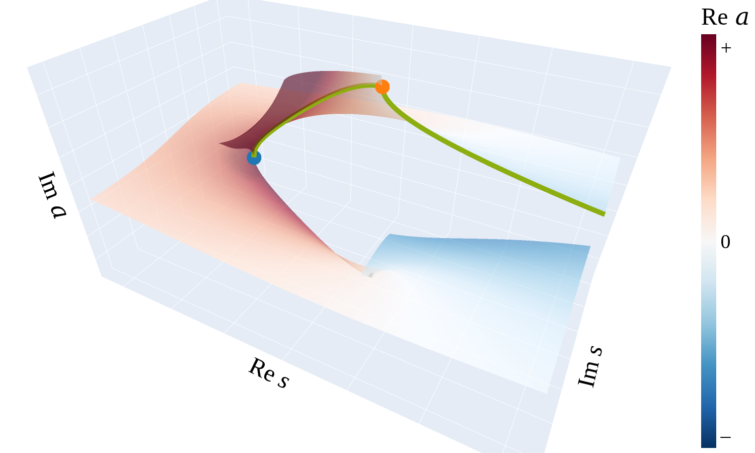