Lifetimes and mixing#
Besides four-momenta, the decay tree contains the information that is needed to simulate decays in flight: production vertices, sampled lifetimes, and the decay mode. Neutral \(B\) mesons also mix, which shows up as an extra node in the tree.
Creating a Generator reads the decay and particle tables and initializes Pythia8, which prints a lot of log output. That output is hidden on this page.
from pyevtgen import Generator

generator = Generator(seed=0)
events = generator.generate("B0", n=20_000)
Lifetimes#
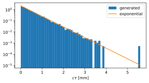
Each unstable particle has a sampled proper decay time lifetime, given as \(c\tau\) in mm. Its distribution is exponential with the mean \(c\tau\) from the particle table:
ctau = np.array([event.lifetime for event in events])
expected = generator.properties("B0").ctau
print(f"sampled mean: {ctau.mean():.4f} mm, table: {expected:.4f} mm")
sampled mean: 0.4597 mm, table: 0.4572 mm
Production vertices#
The position of a particle is its production four-position \((ct, x, y, z)\) in mm. The daughters of a parent that decays at rest are produced at the same point in space, but later in time:
parent:   (0.0, 0.0, 0.0, 0.0)
daughter: (1.2771975199972874, 0.0, 0.0, 0.0)
For a parent in flight, the decay vertex moves along the direction of flight:
mass = generator.properties("B0").mass
p4 = [10.0, 0.0, 0.0, np.sqrt(10.0**2 - mass**2)]
event = generator.decay("B0", p4=p4)
event.daughters[0].position
(0.6893819328762598, 0.0, 0.0, 0.5854691544739364)
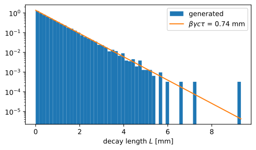
For many decays in flight, the decay length \(L\) follows an exponential distribution with mean \(\beta\gamma c\tau\):
Decay modes#
decay_mode is the index of the decay channel that EvtGen selected from the decay table of the particle. For a \(D^+\), each index corresponds to one set of daughters:
from collections import Counter, defaultdict

d_events = generator.generate("D+", n=20_000)
channels = defaultdict(set)
for event in d_events:
    channels[event.decay_mode].add(" ".join(d.name for d in event.daughters))
for mode, count in Counter(e.decay_mode for e in d_events).most_common(4):
    print(f"{mode:>3}: {count:>5} x {sorted(channels[mode])}")
 32:  1893 x ['K- pi+ pi+']
 12:  1848 x ['anti-K0 mu+ nu_mu']
  1:  1805 x ['anti-K0 e+ nu_e']
 34:  1364 x ['K_L0 pi+ pi0']
Caution
EvtGen delegates many inclusive \(B\) meson decays to Pythia8 through the PYTHIA decay model. Pythia8 resets the selected channel when it replaces the daughters, so all of those decays report decay_mode 0, whatever their daughters are:
b_channels = {
    " ".join(d.name for d in event.daughters)
    for event in events
    if event.decay_mode == 0 and event.daughters[0].name != "anti-B0"
}
len(b_channels)
4834
Mixing#
With the default incoherent mixing (mixing_type=1, see Generator), a neutral \(B^0\) that oscillates before it decays gets a single daughter: an \(\bar{B}^0\) that then decays. The fraction of such events gives the time-integrated mixing probability \(\chi_d\), which is about 0.19:
0.18515
print([daughter.name for daughter in mixed[0].daughters])
['anti-B0']
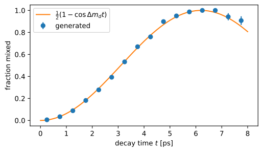
The probability that a \(B^0\) has mixed depends on its decay time as \(\frac{1}{2}\left(1 - \cos\Delta m_d\, t\right)\), with the oscillation frequency \(\Delta m_d \approx 0.5065\,\mathrm{ps}^{-1}\). The sampled lifetimes and the mixing flag of each event reproduce this oscillation:
Coherent mixing (mixing_type=0) is meant for \(B\) meson pairs from \(\Upsilon(4S)\) decays. Because a process can hold only one Generator, the mixing type has to be chosen when the generator is created.