Four-body decays#
A three-body decay of a spin-0 particle has two independent kinematic variables, so a single Dalitz plot shows all of its structure. A four-body decay has five: for instance, two two-body invariant masses and three angles. No single plot shows all of them, so four-body decays are conventionally shown through a set of projections: the invariant masses of all two- and three-particle combinations, and two-dimensional maps of pairs of them.
This page compares \(D^0 \to K^-\pi^+\pi^+\pi^-\) through the resonance cascade \(D^0 \to K^- a_1(1260)^+\), \(a_1^+ \to \rho^0\pi^+\), \(\rho^0 \to \pi^+\pi^-\) with uniform four-body phase space.
Creating a Generator reads the decay and particle tables and initializes Pythia8, which prints a lot of log output. That output is hidden on this page.
from pyevtgen import Generator, final_state_momenta, phase_space

generator = Generator(seed=0)
Generating the samples#
A user decay file forces the cascade. Each intermediate state decays according to its own model, so the resonances shape the four-body final state:
decay_file = Path(mkdtemp()) / "k3pi.dec"
decay_file.write_text("""
Decay D0
1.0 a_1+ K- SVS;
Enddecay
Decay a_1+
1.0 rho0 pi+ VVS_PWAVE 1.0 0.0 0.0 0.0 0.0 0.0;
Enddecay
Decay rho0
1.0 pi+ pi- VSS;
Enddecay
End
""")
generator.read_user_decay_file(decay_file)
events = generator.generate("D0", n=100_000)
[particle.name for particle in events[0].final_state()]
['pi+', 'pi-', 'pi+', 'K-']
The final state is ordered by the decay tree. We reorder it to \((K^-, \pi^+, \pi^+, \pi^-)\), and generate a phase space sample with the same masses and order with phase_space():
order = [3, 0, 2, 1]  # K-, pi+ (from rho), pi+ (from a1), pi-
cascade = final_state_momenta(events)[:, order]

masses = [generator.properties(name).mass for name in ["K-", "pi+", "pi+", "pi-"]]
uniform = phase_space(generator.properties("D0").mass, masses, n=100_000, seed=0)
samples = {"cascade": cascade, "phase space": uniform}
cascade.shape, uniform.shape
EvtMTRandomEngine:Mersenne-Twister random number generator with seed = 1430957218
((100000, 4, 4), (100000, 4, 4))
Invariant mass projections#
The two \(\pi^+\) are identical, so in data one cannot tell which one comes from the \(\rho^0\). Each combination that contains one of them is therefore filled for both pions. The resulting projections cover all two- and three-particle combinations:
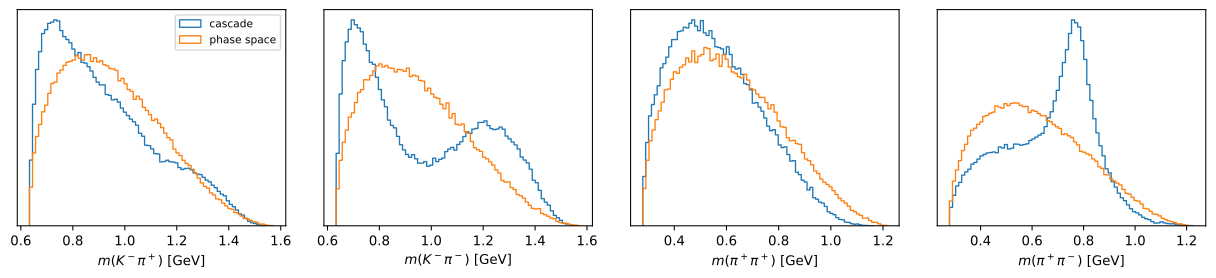
In the two-body masses, the \(\rho^0\) shows up as a peak in \(m(\pi^+\pi^-)\), while the other combinations are only reshaped through the kinematics of the cascade:
plot_projections(2)
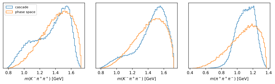
In the three-body masses, the broad \(a_1(1260)^+\) appears in \(m(\pi^+\pi^+\pi^-)\):
plot_projections(3)
Correlations#
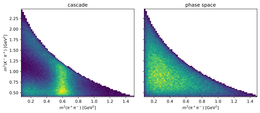
Two-dimensional maps show how the projections are correlated. A natural choice for a four-body decay is a pair of complementary two-body masses, which split the final state into two pairs. Here, \(m^2(\pi^+\pi^-)\) is shown against \(m^2(K^-\pi^+)\) of the other pair, filled for both pion assignments:
The remaining degrees of freedom are angles, for instance the helicity angles of the two pairs in their rest frames and the angle between their decay planes. These are the variables of a full four-body amplitude analysis.